Binary Classification

Introduction

Classification is an important Machine Learning task where an algorithm learns to associate input features to a finite number of classes. For example, given pixels from an animal image as input, output what animal is in that image. Binary classification is a special case where the number of classes is two, for example true or false, good or bad, cat or no cat etc.

I have implemented two binary classification models in TensorFlow, one using simple logistic regression and another using a shallow feedforward neural network (FNN). Logistic regression is a linear classifier, which means that it can only divide input data using a straight line (or plane/hyperplane depending on the dimensionality). Using a FNN with a logistic node as output allows us to divide data using more complex functions. I decided to only use two dimensional data for visualization purposes, but the code can easily be adapted to data with higher dimensionality.

The source code can be found at https://github.com/CarlFredriksson/binary_classification.

Implementation

Import Modules

We will need to import the following modules:

import os
import numpy as np
import tensorflow as tf
import matplotlib as mpl
import matplotlib.pyplot as plt

Generate Data

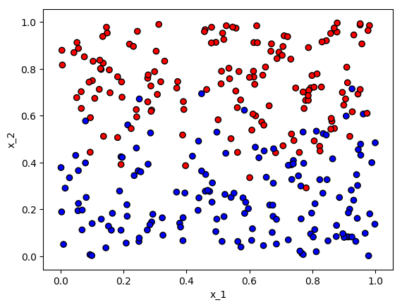
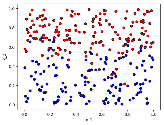
Since this project is only a proof of concept, I decided to use generated training data instead of looking for some real world data. I generated linear data that can be divided using a straight line, and set one side of the line to be class 0 and the other class 1. Some data points had their classes flipped randomly in order to simulate noise that would exist in the real world. Classes were flipped with higher probability for the data points that were close to the boundary line.

def generate_linear_data(num_data_points):
    X = np.random.rand(num_data_points, 2)

    # Set classes with the line x_2 = 0.5 as a boundary
    Y = np.expand_dims([0 if (X[i, 1] > 0.5) else 1 for i in range(num_data_points)], axis=1)

    # Flip the class of the points randomly, with higher probability if the point is close to the boundary
    for i in range(Y.shape[0]):
        distance = abs(X[i, 1] - 0.5)
        flip_prob = max(0, 0.3 - distance)
        if np.random.rand() < flip_prob:
            Y[i] = (Y[i] + 1) % 2

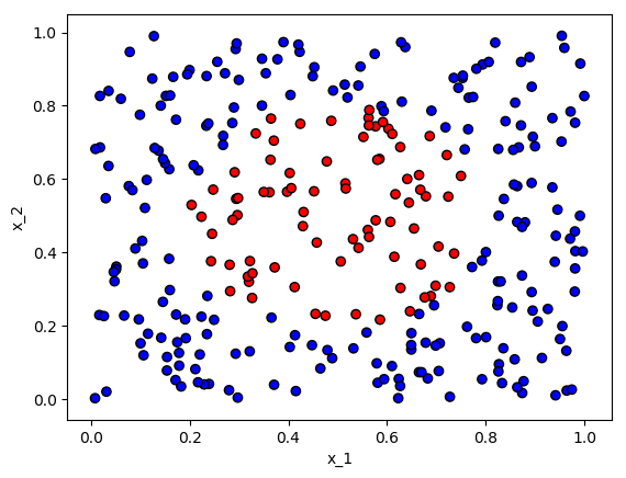
    return X, Y

I also implemented a function for generating non-linear data in the form of a circle. This time I did not bother with adding more noise, since logistic regression will be completely useless on this data set anyway, and it will be sufficient to show the difference between the classification models.

def generate_non_linear_data(num_data_points):
    X = np.random.rand(num_data_points, 2)

    # Set classes with a ring centered at (0.5, 0.5) as a boundary
    Y = np.expand_dims([0 if (np.linalg.norm(X[i] - np.array([0.5, 0.5])) < 0.3) else 1 for i in range(num_data_points)], axis=1)

    return X, Y

Let us generate some training data that will be used to train the models.

Let us also generate some test data that will be used to evaluate the models.

I used the following function to plot the data sets:

def plot_data(X, Y, plot_name):
    colors = Y[:, 0]
    plt.scatter(X[:, 0], X[:, 1], c=colors, cmap=mpl.colors.ListedColormap(["red", "blue"]), edgecolors=["black"])
    plt.xlabel("x_1")
    plt.ylabel("x_2")
    plt.savefig("output/" + plot_name, bbox_inches="tight")
    plt.clf()

Logistic Regression

The first model uses simple logistic regression which outputs $\hat{y} = \sigma(x^T w + b)$, where $\sigma$ is the sigmoid function, $x$ is an input vector, $w$ is a weight vector, and $b$ is a bias vector. We predict class 0 if $\hat{y} <= 0.5$ and class 1 if $\hat{y} > 0.5$. The objective is to find the best decision boundary. A decision boundary separates points in input space where on one side of the boundary one class is predicted, and on the other side another class is predicted. We want a cost function that leads to a decision boundary that predicts the correct class for as many training examples as possible. Let $y \in {0,1}$ be the correct class for a training example $x$, and $\hat{y} = \sigma(x^T w + b)$. The logistic cost function for one training example is:

$$ L(y, \hat{y}) = -(y \log{\hat{y}} + (1 - y) \log{(1 - \hat{y})}) $$

For a training set of many examples we want to compute the average cost. Let $X_{train}$ be the training set with $|X_{train}|$ number of training examples, and $Y_{train}$ the correct classes for those examples. We have the complete logistic cost function:

$$ J(X_{train}, Y_{train}, \hat{y}) = \frac{1}{|X_{train}|} \sum_{x \in X_{train}} L(Y_{train}(x), \hat{y}(x)) $$

The reason for using this cost function instead of the squared error cost, is that it is a convex function which leads to more effective gradient descent.

def logistic_regression_2D(X_train, Y_train, X_test, Y_test, learning_rate, num_epochs, db_plot_name):
    tf.reset_default_graph()

    # Create parameters
    W = tf.get_variable("W", shape=(2, 1), initializer=tf.contrib.layers.xavier_initializer())
    b = tf.get_variable("b", shape=(1, 1), initializer=tf.zeros_initializer())

    # Forward propagation
    X = tf.placeholder(dtype=tf.float32, shape=(None, 2), name="X")
    Y = tf.placeholder(dtype=tf.float32, shape=(None, 1), name="Y")
    Y_hat = tf.sigmoid(tf.matmul(X, W) + b)

    # Compute cost, add small value epsilon to tf.log() calls to avoid taking the log of 0
    epsilon = 1e-10
    J = -tf.reduce_mean(Y * tf.log(Y_hat + epsilon) + (1 - Y) * tf.log(1 - Y_hat + epsilon))

    # Create train op
    optimizer = tf.train.GradientDescentOptimizer(learning_rate)
    train_op = optimizer.minimize(J)

    # Start session
    with tf.Session() as sess:
        # Initialize variables
        sess.run(tf.global_variables_initializer())

        # Training loop
        for i in range(num_epochs):
            sess.run(train_op, feed_dict={X: X_train, Y: Y_train})
            J_train = sess.run(J, feed_dict={X: X_train, Y: Y_train})
            if i%1000 == 0:
                print("i: " + str(i) + ", J_train: " + str(J_train))

        # Evaluate
        J_train = sess.run(J, feed_dict={X: X_train, Y: Y_train})
        J_test = sess.run(J, feed_dict={X: X_test, Y: Y_test})

        # Plot decision boundary
        predict_func = lambda X_grid: sess.run(Y_hat, feed_dict={X: X_grid, Y: Y_train})
        bc_utils.plot_decision_boundary(X_train, Y_train, predict_func, db_plot_name)

        return J_train, J_test

def plot_decision_boundary(X_train, Y_train, predict_func, plot_name):
    interval = np.arange(-0.1, 1.1, 0.001)
    X_1, X_2 = np.meshgrid(interval, interval)
    X_grid = np.c_[X_1.ravel(), X_2.ravel()]
    Y_grid = predict_func(X_grid)
    predictions_grid = np.array([round(x[0]) for x in Y_grid])
    predictions_grid = predictions_grid.reshape(X_1.shape)
    plt.contourf(X_1, X_2, predictions_grid, cmap=mpl.colors.ListedColormap(["#ff6868", "#6875ff"]))
    plt.scatter(X_train[:, 0], X_train[:, 1], c=Y_train[:, 0], cmap=mpl.colors.ListedColormap(["red", "blue"]), edgecolors=["black"])
    plt.savefig("output/" + plot_name, bbox_inches="tight")
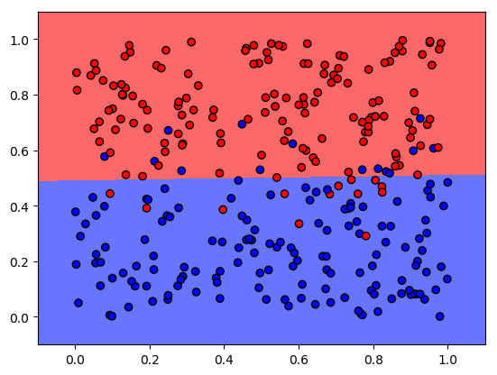
    plt.clf()

As one might expect, this simple model yielded a good result when applied to our generated linear data. The final cost after 20000 epochs and a learning rate of 0.1, was 0.2094 on the training set and 0.2434 on the test set.

As we have already discussed, logistic regression is a linear classifier and should have horrible results on a non-linear data set. This was the case for our generated non-linear data. The algorithm could not find a good decision boundary, and instead predicted the same class for the whole domain. The final cost after 20000 epochs and a learning rate of 0.1, was 0.5892 on the training set and 0.5800 on the test set.

Neural Network Classification

The second model uses a small FNN. The network has two hidden layers with ten neurons each. ReLU is used as an activation function for all layers except the output layer, which uses the sigmoid function. Note that if the hidden layers are removed, we are left with simple logistic regression. I used the same cost function as in the first model.

def nn_binary_classification_2D(X_train, Y_train, X_test, Y_test, learning_rate, num_epochs, db_plot_name):
    tf.reset_default_graph()

    # Create parameters
    W_1 = tf.get_variable("W_1", shape=(2, 10), initializer=tf.contrib.layers.xavier_initializer())
    b_1 = tf.get_variable("b_1", shape=(1, 10), initializer=tf.zeros_initializer())

    W_2 = tf.get_variable("W_2", shape=(10, 10), initializer=tf.contrib.layers.xavier_initializer())
    b_2 = tf.get_variable("b_2", shape=(1, 10), initializer=tf.zeros_initializer())

    W_3 = tf.get_variable("W_3", shape=(10, 1), initializer=tf.contrib.layers.xavier_initializer())
    b_3 = tf.get_variable("b_3", shape=(1, 1), initializer=tf.zeros_initializer())

    # Forward propagation
    X = tf.placeholder(dtype=tf.float32, shape=(None, 2), name="X")
    Y = tf.placeholder(dtype=tf.float32, shape=(None, 1), name="Y")

    Y_hat = tf.matmul(X, W_1) + b_1
    Y_hat = tf.nn.relu(Y_hat)
    Y_hat = tf.matmul(Y_hat, W_2) + b_2
    Y_hat = tf.nn.relu(Y_hat)
    Y_hat = tf.sigmoid(tf.matmul(Y_hat, W_3) + b_3)

    # Compute cost, add small value epsilon to tf.log() calls to avoid taking the log of 0
    epsilon = 1e-10
    J = -tf.reduce_mean(Y * tf.log(Y_hat + epsilon) + (1 - Y) * tf.log(1 - Y_hat + epsilon))

    # Create train op
    optimizer = tf.train.GradientDescentOptimizer(learning_rate)
    train_op = optimizer.minimize(J)

    # Start session
    with tf.Session() as sess:
        # Initialize variables
        sess.run(tf.global_variables_initializer())

        # Training loop
        for i in range(num_epochs):
            sess.run(train_op, feed_dict={X: X_train, Y: Y_train})
            J_train = sess.run(J, feed_dict={X: X_train, Y: Y_train})
            if i%1000 == 0:
                print("i: " + str(i) + ", J_train: " + str(J_train))

        # Evaluate
        J_train = sess.run(J, feed_dict={X: X_train, Y: Y_train})
        J_test = sess.run(J, feed_dict={X: X_test, Y: Y_test})

        # Plot decision boundary
        predict_func = lambda X_grid: sess.run(Y_hat, feed_dict={X: X_grid, Y: Y_train})
        bc_utils.plot_decision_boundary(X_train, Y_train, predict_func, db_plot_name)

        return J_train, J_test

The FNN model also yielded a good result when applied to our generated linear data. The final cost after 20000 epochs and a learning rate of 0.1, was 0.1979 on the training set and 0.2452 on the test set. It did overfit the training set more than the first model as the cost difference between the training set and the test set was greater, and we can see that the decision boundary was not linear. Some overfitting is to be expected since the FNN model is capable of more complex functions, and we did not use any anti-overfitting techniques such as regularization.

The big difference in performance comes when we switch to the non-linear data set. The more flexible FNN model can learn to find an approximately circular decision boundary, and fit the training set very well. The final cost after 20000 epochs and a learning rate of 0.1, was 0.0048 on the training set and 0.1214 on the test set. This time both costs where smaller but the overfitting greater, which can be explained by the relatively small amount of noise in the generated non-linear data, thus allowing a better fit to the training set.

Conclusion

Logistic regression can be a good choice when you are sure that a linear decision boundary will be sufficient. Otherwise you should probably use a neural network or a similarly flexible model. You might have to put in some work in order to find a good network architecture and to avoid overfitting, but the resulting model should have better results on most non-linear data sets.

The source code can be found at https://github.com/CarlFredriksson/binary_classification.

Thank you for reading, and feel free to send me any questions.