Deep Convolutional Generative Adversarial Networks
Introduction
I recently wrote a post about Generative Adversarial Networks (GANs). A Deep Convolutional Generative Adversarial Network (DCGAN) is a type of GAN where the generator is a deep neural network utilizing transpose convolutions and the discriminator is a deep convolutional neural network (CNN). DCGANs were introduced in the paper Unsupervised Representation Learning with Deep Convolutional Generative Adversarial Networks (Radford, Metz, & Chintala, 2016).
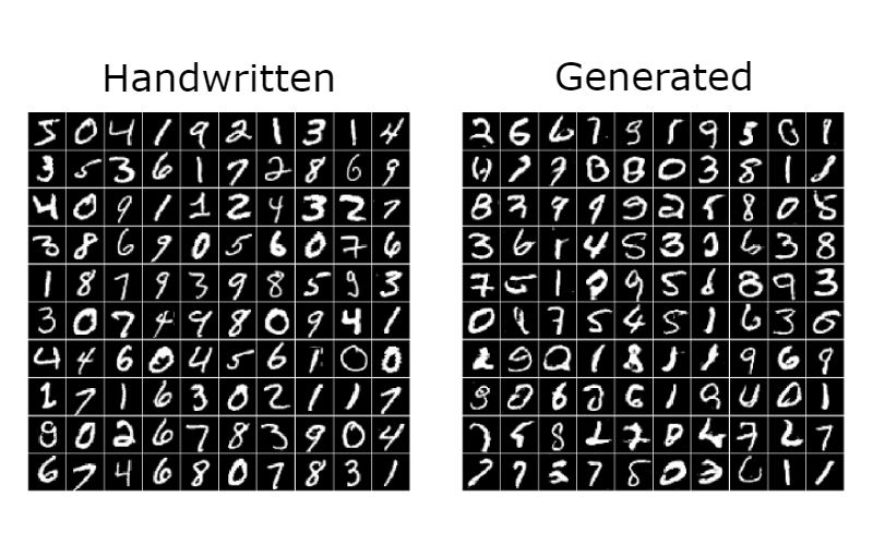
In this post I’m going to show how you can use TensorFlow to implement a DCGAN for generating digits that look handwritten. The dataset I used is the MNIST database of handwritten digits, which I also used in my post about Digit Recognition.
For an introduction to the theory behind DCGANs I refer you to my previous post about Generative Adversarial Networks. The competition between the generator and discriminator remains the same. The generator takes noise as input and generates fake images, and the discriminator tries to distinguish fake images from real images in the training set. We don’t have to change the loss functions, which is a great feature of GANs. The only difference with DCGANs is how the generator and discriminator are implemented.
The source code can be found at https://github.com/CarlFredriksson/dcgan_tensorflow.
Implementation
Import Packages
These are the packages we need to import.
import math
import numpy as np
import tensorflow as tf
import matplotlib.pyplot as plt
import matplotlib.gridspec as gridspec
from tensorflow.keras.datasets import mnist
Load MNIST Data
You could download the dataset from http://yann.lecun.com/exdb/mnist/, but a convenient alternative is to import it from tensorflow.keras.datasets. Since we are doing unsupervised learning we don’t need to store the labels.
X_train = utils.load_mnist_data()def load_mnist_data():
(X_train, _), _ = mnist.load_data()
return X_trainIn order to visualize the data we can plot some examples.
SAMPLE_SIZE = 100utils.plot_sample(X_train[:SAMPLE_SIZE], "output/mnist_data.png")def plot_sample(sample, path):
n = int(np.sqrt(sample.shape[0]))
fig = plt.figure(figsize=(8, 8))
for i in range(n*n):
ax = plt.subplot(n, n, i + 1)
ax.imshow(sample[i], cmap=plt.get_cmap("gray"))
ax.axis("off")
ax.set_xticklabels([])
ax.set_yticklabels([])
fig.subplots_adjust(hspace=0.025, wspace=0.025)
plt.savefig(path, bbox_inches="tight")
plt.clf()
plt.close()
Preprocessing
The generator is going to have a tanh activation at the output layer. Thus we want to normalize the pixel values of the training images from the range $(0,255)$ to $(-1,1)$. We also add a channel dimension of depth 1 since the images were loaded in grayscale.
X_train = utils.preprocess_images(X_train)def preprocess_images(X):
X = X / 255
X = X - 0.5
X = X * 2
X = np.expand_dims(X, axis=-1)
return XPostprocessing
Later we are going to plot samples of generated images and we will need a function that is the inverse of the preprocess function.
def postprocess_images(X):
    X = np.squeeze(X, axis=-1)
    X = X / 2
    X = X + 0.5
    X = X * 255
    return X
Partition Training Data into Mini Batches
The training data is randomly shuffled and partitioned into mini batches.
BATCH_SIZE = 128mini_batches = utils.random_mini_batches(X_train, BATCH_SIZE)def random_mini_batches(X, batch_size):
mini_batches = []
m = X.shape[0]
np.random.shuffle(X)
# Partition into mini-batches
num_complete_batches = math.floor(m / batch_size)
for i in range(num_complete_batches):
batch = X[i * batch_size : (i + 1) * batch_size]
mini_batches.append(batch)
# Handling the case that the last mini-batch < batch_size
if m % batch_size != 0:
batch = X[num_complete_batches * batch_size : m]
mini_batches.append(batch)
return mini_batchesBaseline Model
Let’s start by creating a simple GAN model in order to establish baseline performance. The generator is a simple feedforward neural network (FNN) that takes 100 dimensional noise vectors $Z$ as input, and outputs images with dimensions $(28,28,1)$ and pixel values in the range $(-1,1)$. The discriminator is also a simple FNN that takes images of dimensions $(28,28,1)$ as input and outputs single values representing guesses of whether an input image is real or fake.
def generator(Z):
    with tf.variable_scope("Generator"):
        x = tf.layers.dense(Z, 128, activation="relu")
        x = tf.layers.dense(x, 784, activation="tanh")
        x = tf.reshape(x, [-1, 28, 28, 1])

    return x
def discriminator(X, reuse=False):
with tf.variable_scope("Discriminator", reuse=reuse):
x = tf.layers.flatten(X)
x = tf.layers.dense(x, 128, activation="relu")
x = tf.layers.dense(x, 1, activation="sigmoid")
return xIf you want the rest of the code for the baseline model check out the source code. After training the GAN for 100 epochs I got the following result.

DCGAN Model
Let’s now create a DCGAN model which is better suited for our problem.
Create Generator
The generator takes 100 dimensional noise vectors $Z$ as input and outputs images with dimensions $(28,28,1)$ and pixel values in the range $(-1,1)$. The network architecture is heavily inspired by the architecture guidelines suggested in the original DCGAN paper (Radford, Metz, & Chintala, 2016).
We will use transpose convolutions as a way to do upsampling in a learnable way. Traditional methods of upsampling like nearest-neighbor interpolation or bilinear interpolation are methods without learnable parameters. For generating images we want the network to be able to learn its own upsampling method in order to be able to create convincing fake images.
def generator(Z, is_training):
    with tf.variable_scope("Generator"):
        x = Z
        # x.shape: (?, 1, 1, 100)

        x = tf.layers.conv2d_transpose(x, 256, 7, strides=1, padding="valid", use_bias=False)
        x = tf.layers.batch_normalization(x, training=is_training)
        x = tf.nn.leaky_relu(x)
        # x.shape: (?, 7, 7, 256)

        x = tf.layers.conv2d_transpose(x, 128, 5, strides=2, padding="same", use_bias=False)
        x = tf.layers.batch_normalization(x, training=is_training)
        x = tf.nn.leaky_relu(x)
        # x.shape: (?, 14, 14, 128)

        x = tf.layers.conv2d_transpose(x, 1, 5, strides=2, padding="same")
        x = tf.nn.tanh(x)
        # x.shape: (?, 28, 28, 1)

    return x
Create Discriminator
The discriminator is a CNN that takes images of dimensions $(28,28,1)$ as input and outputs single values representing guesses of whether an input image is real or fake. The network looks like a normal CNN for binary image classification with a few modifications. Most notably, we use strided convolutions instead of pooling layers for downsampling. This is so the network can learn its own downsampling, similarly to the upsampling in the generator.
def discriminator(X, is_training, reuse=False):
    with tf.variable_scope("Discriminator", reuse=reuse):
        x = X
        # x.shape: (?, 28, 28, 1)

        x = tf.layers.conv2d(x, 128, 5, strides=2, padding="same", use_bias=False)
        x = tf.layers.batch_normalization(x, training=is_training)
        x = tf.nn.leaky_relu(x)
        # x.shape: (?, 14, 14, 128)

        x = tf.layers.conv2d(x, 256, 5, strides=2, padding="same", use_bias=False)
        x = tf.layers.batch_normalization(x, training=is_training)
        x = tf.nn.leaky_relu(x)
        # x.shape: (?, 7, 7, 256)

        x = tf.layers.conv2d(x, 1, 7, strides=1, padding="valid")
        x = tf.nn.sigmoid(x)
        # x.shape: (?, 1, 1, 1)

    return x
Create DCGAN
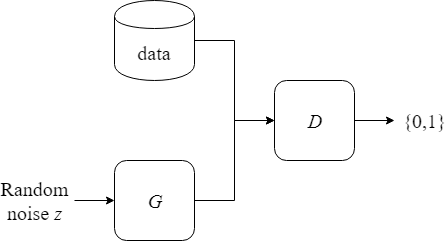
The overall structure is the same as in a regular GAN. The generator $G$ generates fake examples from noise. The discriminator $D$ takes both real examples from training data and fake examples from $G$ as input, and outputs guesses on which examples are real and which are fake.
Note that I used the placeholder is_training mostly out of habit. It’s going to be set to true for both training and generation of images. When doing supervised learning there is a clear distinction between training a model and using it for inference. When batch normalization layers are applied during training, the normalization step is done using mean and variance of the current mini-batch. When doing inference, the normalization step uses population mean and population variance instead, which are statistics estimated during training using moving mean and variance.
Since we are generating new data from noise and not doing any inference, there is no need to change the batch norm layers from training mode to inference mode. I tried both and found that keeping training mode on worked the best. When images where generated with inference mode on (is_training set to false) they were slightly blurry, and more importantly they ended up generating the same number (9) in most cases.
NOISE_DIM = 100X = tf.placeholder(tf.float32, shape=(None, X_train.shape[1], X_train.shape[2], X_train.shape[3]))
Z = tf.placeholder(tf.float32, [None, 1, 1, NOISE_DIM])
is_training = tf.placeholder(tf.bool, shape=())
G, D_real, D_fake = create_gan(X, Z, is_training)def create_gan(X, Z, is_training):
G = generator(Z, is_training)
D_real = discriminator(X, is_training)
D_fake = discriminator(G, is_training, reuse=True)
return G, D_real, D_fakeCreate Training Steps
Just like in a regular GAN we will use separate training steps for the generator and discriminator. We will also use the same loss functions as in a regular GAN. As suggested in the DCGAN paper, we will use Adam optimizers with parameters $\beta_1$ and learning rate set to 0.5 and 0.0002 respectively.
BETA1 = 0.5
LEARNING_RATE = 0.0002G_loss_func, D_loss_func = utils.create_loss_funcs(D_real, D_fake)
G_vars = tf.get_collection(tf.GraphKeys.GLOBAL_VARIABLES, scope="Generator")
D_vars = tf.get_collection(tf.GraphKeys.GLOBAL_VARIABLES, scope="Discriminator")
G_train_step = tf.train.AdamOptimizer(learning_rate=LEARNING_RATE, beta1=BETA1).minimize(G_loss_func, var_list=G_vars)
D_train_step = tf.train.AdamOptimizer(learning_rate=LEARNING_RATE, beta1=BETA1).minimize(D_loss_func, var_list=D_vars)def create_loss_funcs(D_real, D_fake):
eps = 1e-12
G_loss_func = tf.reduce_mean(-tf.log(D_fake + eps))
D_loss_func = tf.reduce_mean(-(tf.log(D_real + eps) + tf.log(1 - D_fake + eps)))
return G_loss_func, D_loss_funcTrain Model
I trained the model for 20 epochs and plotted a sample of generated images after each epoch.
NUM_EPOCHS = 20# Start session
with tf.Session() as sess:
sess.run(tf.global_variables_initializer())
# Training loop
for epoch in range(NUM_EPOCHS):
for X_batch in mini_batches:
Z_batch = utils.generate_Z_batch((X_batch.shape[0], 1, 1, NOISE_DIM))
# Compute losses
G_loss, D_loss = sess.run([G_loss_func, D_loss_func], feed_dict={X: X_batch, Z: Z_batch, is_training: True})
print("Epoch [{0}/{1}] - G_loss: {2}, D_loss: {3}".format(epoch, NUM_EPOCHS - 1, G_loss, D_loss))
# Run training steps
_ = sess.run(G_train_step, feed_dict={Z: Z_batch, is_training: True})
_ = sess.run(D_train_step, feed_dict={X: X_batch, Z: Z_batch, is_training: True})
# Plot generated images
Z_batch = utils.generate_Z_batch((SAMPLE_SIZE, 1, 1, NOISE_DIM))
gen_imgs = sess.run(G, feed_dict={Z: Z_batch, is_training: True})
gen_imgs = utils.postprocess_images(gen_imgs)
utils.plot_sample(gen_imgs, "output/dcgan/dcgan_gen_data_" + str(epoch) + ".png")def generate_Z_batch(size):
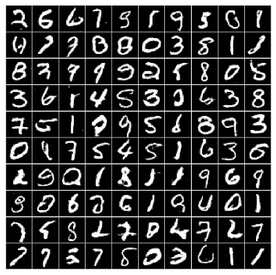
return np.random.uniform(low=-1, high=1, size=size)Images generated after the 20th epoch:
Conclusion
This was a fun project and I’m happy about how it turned out. Not all of the generated images could fool a human, but most of them look like they could be handwritten digits to me. Although generating handwritten digits is not the most exiting objective, it serves as a good introductory task for learning how to implement and tune DCGANs.
Thank you for reading and feel free to send me any questions.