Generative Adversarial Networks

Introduction

Generative Adversarial Networks (GANs) have been getting a lot of attention recently. They have been used for many different tasks, such as generating anime characters (Jin et al., 2017, https://arxiv.org/abs/1708.05509), generating photos of fake celebrities (Karras, Aila, Laine, & Lehtinen, 2017, https://arxiv.org/abs/1710.10196), increasing resolution in photos (Ledig et al., 2016, https://arxiv.org/abs/1609.04802), and general image-to-image translation (Isola, Yan Zhu, Zhou, Efros, 2017, https://arxiv.org/abs/1611.07004).

GANs were introduced in (Goodfellow et al., 2014, https://arxiv.org/abs/1406.2661) as an unsupervised learning model, trained on data without labels. The model learns to take noise as input and output data that resembles examples from the training set. There are versions of GANs that can utilize additional information as input, such as conditional GANs (CGANs), but in this post I’m going to focus on the basic version.

I’m going to explain some of the theory behind GANs and then show how you can implement a simple version in TensorFlow. The source code can be found at https://github.com/CarlFredriksson/gan_tensorflow.

Theory

A GAN consists of two parts, a generator $G$ and a discriminator $D$. The objective for $G$ is to take random noise $z$ as input and generate a fake example that looks like it comes from the real training data. The objective for $D$ is to take an example $x$ from the training data or a fake example $G(z)$ as input and output either 0 or 1. If the example is from the training data $D$ should output 1, and if the example is fake $D$ should output 0. In other words, $D$ is a binary classifier on whether the input is real (part of the training data) or fake (generated by $G$).

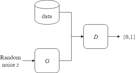
Note that $G$ is what we are ultimately interested in. After training, $G$ is what we will use in our applications to generate new data. $D$ is there to help train $G$. Training using an adversary in this way is a powerful idea that lets us define simple loss functions for $G$ and $D$ that don’t need to be changed between different tasks. GANs remove the need for handcrafting specific loss functions for many problems.

Minimax Game

$G$ and $D$ have directly competing objectives, and the situation can be modelled as a minimax zero-sum game where $G$ and $D$ are the players. When $G$ learns to create better fakes, it forces $D$ to get better at detecting them and vice versa. The competition makes $G$ and $D$ better and better until a steady state is reached.

An analogy could be a cop vs a criminal making counterfeit money. As the cop gets better at detecting fake bills, the criminal has to learn more complex counterfeiting methods, which in turn forces the cop to get even better, and so on.

The game that $G$ and $D$ plays can be modelled by the value function $V(D,G)$:

$$ \underset{G}{min} \thinspace \underset{D}{max} \thinspace V(D,G) = \mathbb{E}_{x \sim p_{data}(x)}[log \thinspace D(x)] + \mathbb{E}_{z \sim p_{z}(z)}[log(1 - D(G(z)))] \tag 1 $$

Training

One training step consists of:

• Sample a mini batch of $m$ noise vectors ${z^{(1)},\dots,z^{(m)}}$
• Sample a mini batch of $m$ training examples ${x^{(1)},\dots,x^{(m)}}$
• Update $D$ by doing one gradient descent step on its loss function:

$$ J_D = - \frac{1}{m} \sum_{i=1}^{m} \Big[log \thinspace D\big(x^{(i)}\big) + log\big(1 - D\big(G\big(z^{(i)}\big)\big)\big)\Big] \tag 2 $$

• Update $G$ by doing one gradient descent step on its loss function:

$$ J_G = - \frac{1}{m} \sum_{i=1}^{m} \Big[log \thinspace D\big(G\big(z^{(i)}\big)\big)\Big] \tag 3 $$

I chose to minimize $-log \thinspace D(G(z))$, rather than $log(1 - D(G(z)))$. This is suggested in the original GAN paper to provide stronger gradients for $G$ early in training, while keeping the same fixed point dynamics of $G$ and $D$ as in equation 1. Since the performance of $G$ is poor in the early stages, $D$ can easily distinguish fake examples from real training data, which results in small gradients for $G$. If needed, the imbalance can be combated further by slowing down the learning of $D$. This can be done by running more than one training step for $G$ for every step of $D$ or lowering the learning rate of $D$.

Implementation

Let us now implement a GAN. I chose to keep it simple in order to focus on the basic ideas. We are going to generate a two-dimensional dataset using a quadratic function, and implement $G$ and $D$ as small feedforward neural networks (FNNs).

Import Packages

These are the packages we need to import.

import math
import numpy as np
import tensorflow as tf
import matplotlib.pyplot as plt

Generate Data

The data is generated using the function $y=x^2 + 5$. The data contains two-dimensional points without labels that are shuffled and partitioned into mini-batches for training.

data = generate_data()
plot_data(data)
mini_batches = random_mini_batches(data, BATCH_SIZE)

def generate_data(n=1000, scale=10):
    X = scale*(np.random.random_sample(n) - 0.5)
    Y = X**2 + 5

    return np.array([X, Y]).T

def plot_data(data):
    plt.plot(data[:, 0], data[:, 1], "o")
    plt.savefig("output/data.png", bbox_inches="tight")
    plt.clf()

def random_mini_batches(data, batch_size):
    mini_batches = []
    m = data.shape[0]
    np.random.shuffle(data)

    # Partition into mini-batches
    num_complete_batches = math.floor(m / batch_size)
    for i in range(num_complete_batches):
        batch = data[i * batch_size : (i + 1) * batch_size]
        mini_batches.append(batch)

    # Handling the case that the last mini-batch < batch_size
    if m % batch_size != 0:
        batch = data[num_complete_batches * batch_size : m]
        mini_batches.append(batch)

    return mini_batches

Create Model

It is time to create the GAN. Let’s start by defining two placeholders X and Z. X is the placeholder for batches of training data, and Z is the placeholder for batches of random noise.

X = tf.placeholder(tf.float32, [None, 2])
Z = tf.placeholder(tf.float32, [None, 2])

Let’s create two functions for defining the generator $G$ and the discriminator $D$.

def generator(Z, hidden_sizes=[10, 10]):
    with tf.variable_scope("GAN/Generator"):
        h1 = tf.layers.dense(Z, hidden_sizes[0], activation=tf.nn.leaky_relu)
        h2 = tf.layers.dense(h1, hidden_sizes[1], activation=tf.nn.leaky_relu)
        out = tf.layers.dense(h2, 2)

    return out

def discriminator(X, hidden_sizes=[10, 10], reuse=False):
    with tf.variable_scope("GAN/Discriminator", reuse=reuse):
        h1 = tf.layers.dense(X, hidden_sizes[0], activation=tf.nn.leaky_relu)
        h2 = tf.layers.dense(h1, hidden_sizes[1], activation=tf.nn.leaky_relu)
        out = tf.layers.dense(h2, 1, activation=tf.nn.sigmoid)

    return out

Using our generator and discriminator functions, we can create the GAN model. The tensors we are interested in is the output of $G$, the output of $D$ when real training data is used as input, and the output of $D$ when the input is generated fakes from $G$. The reuse flag is set to true when we call the discriminator function for the second time, since we only want one set of variables for $D$.

gen_out, disc_out_real, disc_out_fake = create_model(X, Z)

def create_model(X, Z):
    gen_out = generator(Z)
    disc_out_real = discriminator(X)
    disc_out_fake = discriminator(gen_out, reuse=True)

    return gen_out, disc_out_real, disc_out_fake

Train Model

To train the model we need to create loss functions, which are defined in equations 2 and 3. Note the addition of the small value EPS in order to avoid taking the log of 0.

EPS = 1e-12

disc_loss = tf.reduce_mean(-(tf.log(disc_out_real + EPS) + tf.log(1 - disc_out_fake + EPS)))
gen_loss = tf.reduce_mean(-tf.log(disc_out_fake + EPS))

Since we are alternating between training $G$ and $D$, we need to create a separate training step for each.

LEARNING_RATE = 0.001

gen_vars = tf.get_collection(tf.GraphKeys.GLOBAL_VARIABLES, scope="GAN/Generator")
disc_vars = tf.get_collection(tf.GraphKeys.GLOBAL_VARIABLES, scope="GAN/Discriminator")

gen_train_step = tf.train.AdamOptimizer(learning_rate=LEARNING_RATE).minimize(gen_loss, var_list=gen_vars)
disc_train_step = tf.train.AdamOptimizer(learning_rate=LEARNING_RATE).minimize(disc_loss, var_list=disc_vars)

Now we are ready to train the model. The performance of the generator is plotted every 250th epoch, and some of the results for one training run can be seen below.

NUM_EPOCHS = 5000
BATCH_SIZE = 32

# Start session
with tf.Session() as sess:
    sess.run(tf.global_variables_initializer())

    # Training loop
    for epoch in range(NUM_EPOCHS):
        for X_batch in mini_batches:
            Z_batch = generate_Z_batch(X_batch.shape[0])
            _, disc_loss_train = sess.run([disc_train_step, disc_loss], feed_dict={X: X_batch, Z: Z_batch})
            _, gen_loss_train = sess.run([gen_train_step, gen_loss], feed_dict={Z: Z_batch})
        if (epoch % 250) == 0:
            print("Epoch " + str(epoch) + " - plotting generated data")
            plot_generated_data(data, lambda Z_batch: sess.run(gen_out, feed_dict={Z: Z_batch}), epoch)

    print("Training finished - plotting generated data")
    plot_generated_data(data, lambda Z_batch: sess.run(gen_out, feed_dict={Z: Z_batch}), NUM_EPOCHS - 1)

def plot_generated_data(data, gen_func, epoch):
    Z_batch = generate_Z_batch(data.shape[0])
    gen_data = gen_func(Z_batch)
    plt.plot(data[:, 0], data[:, 1], "o")
    plt.plot(gen_data[:, 0], gen_data[:, 1], "o")
    plt.title("Epoch " + str(epoch))
    plt.savefig("output/gen_data_" + str(epoch) + ".png", bbox_inches="tight")
    plt.clf()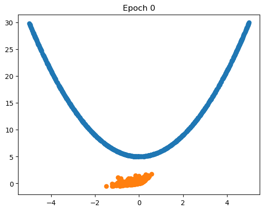

After 5000 epochs, $G$ has learned to generate data points that resemble the training data pretty well.

Conclusion

GANs are based on the idea of adversarial learning, and are capable of incredible performance on a wide variety of problems. In order to focus on the basic properties of GANs, this post showed how to implement a simple GAN and apply it on a simple task. I urge you to check out some of the recent papers to see really cool applications of GANs if you haven’t already.

I hope this post was useful to you, and feel free to send me any questions.