Markov Decision Processes
Introduction
A Markov decision process (MDP) is a mathematical formalization of a sequential decision-making process where actions affect both immediate reward and the next state. MDPs are similar to Multi-armed Bandits in that the agent repeatedly has to make decisions and receives immediate rewards depending on what action is selected. What makes MDPs more complex is that the actions affect the subsequent states, and thus affect future rewards as well. The goal of the agent is the same, to maximize expected return (expected cumulative future reward). In an MDP, each state could have different actions available. After an agent selects an action, the environment gives the agent a reward and presents a new state. Figure 3.1 from Reinforcement Learning: An Introduction (Sutton, Barto, 2018) illustrates the interaction between agent and environment.

At each time step $t=0,1,2,…$, the agent observes a representation of the environment’s state $S_t \in \mathcal{S}$, where $\mathcal{S}$ is the set of all states that aren’t terminal states (the set $\mathcal{S}^+$ includes all terminal states). The agent selects an action $A_t \in \mathcal{A}(S_t)$, where $\mathcal{A}(S_t)$ is the set of all available actions in state $S_t$. The next time step, the agent receives a numerical reward $R_{t+1} \in \mathcal{R} \subset \mathbb{R}$ that depends on the previous state and selected action. The agent observes a new state $S_{t+1}$ and the process continues. This process creates a sequence (or trajectory) of the following form:
$$ S_0,A_0,R_1,S_1,A_1,R_2,S_2,A_2,R_3,… $$
Dynamics Function $p$
This article is going to focus on finite MDPs, which are MDPs where the sets $\mathcal{S}, \mathcal{A}, \mathcal{R}$ all have a finite number of elements. Finite MDPs are defined by their dynamics function $p$:
$$ p(s^\prime,r|s,a) = Pr{S_t=s^\prime, R_t=r | S_{t-1}=s, A_t=a} $$
In other words, $p$ defines the joint probability of observing state $s^\prime$ and receiving reward $r$ after being in state $s$ and taking action $a$.
Episodic and Continuous Tasks
MDPs can be divided into episodic and continuous tasks. Episodic tasks have a clear ending, the agent will eventually reach a terminal state. Continuous tasks have no clear ending and potentially continue forever. In both type of tasks the goal is to maximize expected return. However, the return can be defined in different ways.
The return is denoted $G_t$ and the final time step is denoted $T$. In episodic tasks, $T$ is finite and $G_t$ can be defined as:
$$ G_t = R_{t+1} + R_{t+2} + R_{t+3} + … + R_{T} = \sum_{k=t+1}^{T} R_k $$
In continuous tasks, $T = \infty$ and $G_t$ could easily diverge. To make $G_t$ converge we add add a parameter $0 \leq \gamma \leq 1$, called the discount rate:
$$ G_t = R_{t+1} + \gamma R_{t+2} + \gamma^2 R_{t+3} + … = \sum_{k=0}^{\infty} \gamma^k R_{t+k+1} $$
This is called discounting and means that rewards closer to the current time step will be prioritized. We can also define the return in a way that works for both episodic and continuous tasks:
$$ G_t = \sum_{k=t+1}^{T} \gamma^{k-t-1} R_k $$
When the task is episodic we usually set $\gamma = 1$ (sometimes it might make sense to use discounting for an episodic task). When the task is continuous we usually set $\gamma < 1$.
Examples
A wide array of problems can be formulated as MDPs. Some examples:
- Chess: The states are the position of the pieces. Rewards are 0 except when reaching a terminal state (win, draw, loss). A reward of 1 is given for a win, 1/2 for a draw, and 0 for a loss. The actions are all legal moves in a given state and they deterministically change the state. Since there are terminal states that eventually will be reached it is an episodic task.
- Cleaning robot: The states are combinations of the robots sensor readings, such as position and dust-detection sensors. Positive rewards are given when dust is cleaned up. You might also add a negative reward when the robot runs out of battery, to incentivize the robot to go to its recharging station before running out. The actions could be on the abstraction level of activating motors, or higher level like “move right”. Could be modelled either as an episodic or continuous task, depending on if you want the robot to run all the time or not.
- Temperature control: The states are temperature readings on a thermometer. Negative reward is given when a human manually has to adjust the temperature. The actions are how much power to send to different radiators. Will probably be a continuous task.
Note the importance of designing good rewards, such that if the agent learns to optimize expected return, it will also perform the task very well.
Solving MDPs
The objective of the agent is to maximize expected cumulative future reward. In other words, we want to find a policy that gives the agent as much expected return as possible. A policy is a mapping from states to probabilities of selecting each available action in that state. Solving an MDP usually means finding an optimal policy. When MDPs are small (the sets of states and actions are small) and the dynamics function $p$ is fully known, we can find the optimal policy by solving the Bellman equations, more on this later. MDPs are often too big for this to be computationally feasible. There is a collection of algorithms called dynamic programming (DP) that can be more efficient at finding the optimal policy. When the MDPs are too large for DP or when the dynamics function is not explicitly known (which is often the case for real world appplications), we use reinforcement learning (RL) instead. In RL the aim is usually to find a policy that is good but doesn’t have to be optimal.
The aim of this article is to introduce the basics of finite MDPs. To read more about this subject, I recommend the aforementioned (Sutton, Barto, 2018).
Policies and Value Functions
As mentioned above, a policy is a mapping from states to probabilities of selecting each available action in that state. More formally, if the agent is following policy $\pi$ at time $t$, then $\pi(a|s)$ is the probability that $A_t=a$ if $S_t=s$. A special case is deterministic policies where we denote the action that will be selected in state $s$ by $\pi(s)$.
Value functions are functions that map states, or state-action pairs, to expected return when following a specific policy $\pi$. You can think of value functions as how good a state, or state-action pair, is when following $\pi$. Value functions often can’t be computed exactly, but estimating them and using the estimates to make policy decisions is a part of almost all RL algorithms. There are two types of value functions, state-value functions and action-value functions.
The state-value function of a state $s$ when following policy $\pi$, denoted $v_{\pi}(s)$, is the expected return when following $\pi$ from $s$. More formally:
$$ v_{\pi}(s) = E_{\pi}[G_t | S_t=s] = E_{\pi}\Big[\sum_{k=t+1}^{T} \gamma^{k-t-1} R_k \Big| S_t=s \Big] $$
The action-value function of a state $s$ and action $a$ when following policy $\pi$, denoted $q_{\pi}(s,a)$, is the the expected return when taking action $a$ in $s$, and then following $\pi$ from the new state. More formally:
$$ q_{\pi}(s,a) = E_{\pi}[G_t | S_t=s, A_t=t] = E_{\pi}\Big[\sum_{k=t+1}^{T} \gamma^{k-t-1} R_k \Big| S_t=s, A_t=a \Big] $$
A policy $\pi$ is better than or equal to policy $\pi^\prime$ if its expected return is greater than or equal to that of $\pi^\prime$ for all states. More formally, $\pi \geq \pi^\prime$ if and only if $v_{\pi}(s) \geq v_{\pi^\prime}(s)$ for all states $s$. There is always at least one optimal policy, and we denote all of them $\pi_*$. Even though there can be multiple optimal policies, they all share the same optimal state-value function, defined as $v_*(s)=\max_{\pi} v_{\pi}(s)=v_{\pi_*}(s)$. They also share the same optimal action-value function, defined as $q_*(s,a)=\max_{\pi} q_{\pi}(s,a)=q_{\pi_*}(s,a)$.
Bellman Equations
An important property of value functions that is used throughout RL and DP is that they are recursive. We can use this property to define Bellman equations. Lets’ start with the Bellman equation for $v_{\pi}$:
$$ v_{\pi}(s) = \sum_a \pi(a|s) \sum_{s^\prime,r} p(s^\prime,r|s,a) \big(r + \gamma v_{\pi}(s^\prime) \big) $$
Derivation:
Let’s continue with the Bellman equation for $q_{\pi}$:
$$ q_{\pi}(s,a) = \sum_{s^\prime,r} p(s^\prime,r|s,a) \big(r + \gamma \sum_{a^\prime} \pi(a^\prime|s^\prime) q(a^\prime,s^\prime) \big) $$
Derivation:
We can do the same thing for the optimal value functions. These are sometimes called Bellman optimality equations. Let’s start with the Bellman equation for $v_*$:
Derivation:
Let’s continue with the Bellman equation for $q_*$:
Derivation:
The equations must hold for all states, thus we have systems of linear equations we can solve to compute value functions. In the optimal case it is a bit trickier since they involve the non-linear operation max. The systems of non-linear equations can still be solved to compute the optimal value functions. Even though it is theoretically possible to solve the Bellman equations for all finite MDPs where the dynamics function is known, it becomes very computationally expensive as MDPs get larger.
If you know an optimal value function, it’s trivial to compute the optimal policy. If you have the optimal state-value function, simply look one step ahead in every state and select actions greedily. In other words, select actions by:
If you have the optimal action-value function it is even easier. In all states, simply select the action with the highest action-value function:
If there are ties between actions in either case, you can select any probability distribution between the tying actions.
Gridworld Example
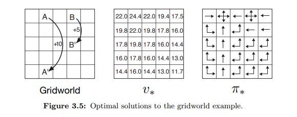
Gridworlds are often used as examples of MDPs. Example 3.5 from (Sutton, Barto, 2018) is a simple example of a finite MDP. The left part of figure 3.2 from (Sutton, Barto, 2018) shows the gridworld. Each cell is a state and the agent can select between the actions: north, south, east, and west in all states. The actions deterministically move the agent in their respective directions, except when they would move the agent out of the grid. In that case the state will remain unchanged and the agent will receive a reward of -1. When the agent selects any action in state $A$, it will be moved to state $A^\prime$ and receive a reward of +10. When the agent selects any action in state $B$, it will be moved to state $B^\prime$ and receive a reward of +5. In all other cases the agent will receive a reward of 0.

The right part of figure 3.2 shows the state-value function $v_{\pi}$ for the policy where all actions are selected at random with equal probability in all states. Since there is no terminal state, discounting was used with rate $\gamma=0.9$. The authors of the book solved the Bellman equations to compute the value function.
The authors also solved the Bellman equations for $v_*$, and the optimal state-value function can be seen in the middle of figure 3.5 from (Sutton, Barto, 2018). The right part shows the corresponding optimal policies $\pi_*$. When there are multiple arrow-directions in a state, it means that any of those directions is an optimal action in that state.
Conclusion
This has been a short introduction to MDPs. The formalization is pretty simple but can model a great deal of problems and is fundamental to the majority of reinforcement learning.
Thank you for reading and feel free to send me any questions.