Multi-armed Bandits

Introduction

A multi-armed bandit problem is a problem where an agent repeatedly has to make a choice between actions that give the agent rewards. Each action has a different probability distribution that determines how much reward is given, and these distributions are not known to the agent. The objective of the agent is to maximize expected cumulative future reward, which is called expected return. The name multi-armed bandit comes from slot machines (one-armed bandits) and one can imagine the actions the agent takes as choosing which arm to pull on a slot machine with multiple arms.

Let’s say we have a $k$-armed bandit problem, with $k$ actions $a$. We can denote the action selected at time $t$ as $A_t$, and the reward received as $R_t$. The value of an action, $q_*(a)$, is defined as the expected reward given that $a$ is selected:

$$ q_*(a) = E[R_t|A_t=a] $$

If the agent knew the actual value for each action, it would be trivial to solve the problem by simply selecting the action with the highest value all the time. Instead the agent has to estimate the value of each action. We denote the estimate of the value of selecting action $a$ at time $t$ as $Q_t(a)$. If the agent’s value estimates are perfect, it can make perfect decisions, so we want $Q_t(a)$ to be as close to $q_*(a)$ as possible.

A bandit problem is a simple version of Reinforcement Learning (RL) problems. In full RL problems, the agent similarly want to maximize expected return, but the selected actions also affect the state of the agent’s environment which affects future rewards and makes the problem more complicated. Even though bandit problems are simpler, studying them provides a good base for understanding many aspects of RL.

There is a type of bandit problem called contextual bandits where state has to be taken into account. For example you can imagine a problem with multiple $k$-armed bandits and each time step the agent is presented with a random one among them. The agent also receives some clue about what the current bandit is and can learn a policy. A policy is a mapping from states to probability distributions over actions that determines what action to take in any given state. Contextual bandits are closer to full RL problems since they have states, but are still simpler since actions does not affect future states.

The aim of this article is to introduce the basics of multiple-armed bandit problems. To read more about this subject, I recommend Reinforcement Learning: An Introduction (Sutton, Barto, 2018). The source code can be found at https://github.com/CarlFredriksson/multi_armed_bandits.

Value Estimation

To estimate the value of each action we can set our estimates to an initial value $Q_0$ and then update the estimate for an action every time the agent takes that action. The general update rule is as follows:

$$ Q_{t+1}(a) = Q_t(a) + \alpha (R_t - Q_t(a)) $$

This update rule brings the estimate closer to the most recently observed reward $R_t$. How much the estimate should move towards the reward depends on $\alpha$, which is called the step size. The step size can be a constant or be computed in various ways. One of the more natural ways to compute $\alpha$ is to set it to $1/N(a)$, where $N(a)$ is the number of times action $a$ has been selected. This step size means that the value estimates will be the average reward received when taking that action. To see that this is the case we can let $Q_{n+1}(a)$ be the average of all received rewards when selecting action $a$ and manipulate the expression. For brevity, assume that we are looking at a single action and drop the $a$. Let $Q_{n}=Q_{n}(a)$, $n=N(a)$, and $R_n$ be the reward received when taking the action the $n$-th time:

Thus with $\alpha = 1/N(a)$, the estimate $Q_{t}(a)$ will be the average of all received rewards and will converge to the real value $q_*(a)$ by the law of large numbers. This step size is very good when the problem is stationary, in other words, when $q_*(a)$ stays the same for all $t$. However, when the problem is non-stationary and $q_*(a)$ changes, $\alpha = 1/N(a)$ might not lead to good estimates in the long term. This is because the observed rewards affect the estimates less and less the more times actions gets selected. In other words, $Q_{t}(a)$ will change less as time goes on. When the problem is non-stationary it is more appropriate to use a constant $\alpha \in (0,1]$. This leads to recent rewards affecting the estimates more than older ones, with the extreme $\alpha = 1$ leading to estimates only caring about the most recent reward. Thus a constant $\alpha$ will make the agent more adaptable to changing $q_*(a)$.

Action Selection

Now we have discussed a couple of options for estimating the value of actions, but how should the agent select actions? The first thing that comes to mind is probably to be greedy and simply select the action with the highest estimated value. In other words, the agent exploits its current knowledge in order to get as much immediate reward as possible. This is an important part of action selection since the objective is to maximize expected return. However, if an agent is too greedy and only exploits, it might not learn accurate value estimates. If an agent has inaccurate value estimates, it can select a sub-optimal action when it exploits. This is why the opposite of exploitation, exploration, is also important when selecting actions.

Exploration is the act of sacrificing immediate reward for gaining knowledge about the problem, in this case to get better value estimates. There is an important tradeoff in RL (and many other fields) called exploration versus exploitation. This is a tradeoff because an agent can’t do both at the same time. The tradeoff needs to be balanced, since if the agent exploits too much it might take a long time to learn what the best action is, or it might never learn it. On the other hand, if the agent explores too much it will miss out on a lot of reward from selecting sub-optimal actions.

There are many methods for balancing the tradeoff. One of the simpler ones is $\epsilon$-greedy, which means that the agent is greedy with probability $1-\epsilon$, and selects a random action with probability $\epsilon$.

Action-value Methods

When a method for value estimation is combined with a method for action selection it is called an action-value method. To roughly assess the performance of different action-value methods we can use a set of randomly generated $k$-armed bandit problems.

The code below generates multiple bandit problems with different values $q_*(a)$. It runs $\epsilon$-greedy and greedy only methods ($\epsilon$-greedy with $\epsilon=0$) with different parameter settings on the generated problems. The results are averaged over the generated problems and plots of both reward over time and percentage of optimal action selected over time are saved. The same procedure is also done for the non-stationary case, when $q_*(a)$ changes over time.

import numpy as np
import matplotlib.pyplot as plt
import math

def my_argmax(Q_values):
    """
    Returns the index of the maximum value in Q_values.
    In case of ties, one of the tying indices are selected at uniform-random and returned.
    """
    max_val = -math.inf
    ties = []
    for i in range(len(Q_values)):
        Q_val = Q_values[i]
        if Q_val > max_val:
            max_val = Q_val
            ties = [i]
        elif Q_val == max_val:
            ties.append(i)

    return np.random.choice(ties)

def run_epsilon_greedy(q, num_steps, epsilon, const_alpha=None, Q_0=0, stationary=True):
    """
    Run a single run of the epsilon greedy algorithm.
    Returns the returns and an array where 1 means optimal action was selected and 0 it wasn't.
    """
    R = np.zeros((num_steps,))
    optimal = np.zeros((num_steps,))
    Q = np.ones(np.shape(q)) * Q_0
    N = np.zeros(np.shape(q))

    # Run steps
    for t in range(0, num_steps):
        if not stationary:
            q = q + np.random.normal(scale=0.05, size=np.shape(q))

        # Choose action greedily by default and randomly by probability epsilon
        a = my_argmax(Q)
        if np.random.uniform(low=0.0, high=1.0) < epsilon:
            a = np.random.randint(low=0, high=len(Q) - 1)
        N[a] += 1
        if a == np.argmax(q):
            optimal[t] = 1

        # Get reward
        R[t] = np.random.normal(loc=q[a])

        # Update Q
        alpha = const_alpha
        if const_alpha is None:
            alpha = 1 / N[a]
        Q[a] = Q[a] + alpha * (R[t] - Q[a])

    return R, optimal

def run_experiments(parameters, num_runs, num_steps, k, stationary=True):
    """
    Run multiple runs of epsilon greedy.
    Returns the averaged results and optimal action selections.
    """
    bandits = np.random.normal(loc=0, scale=1, size=(num_runs, k))
    R = np.zeros((len(parameters), num_runs, num_steps))
    optimal = np.zeros(np.shape(R))

    for i in range(len(parameters)):
        for j in range(num_runs):
            if j % 100 == 0:
                print("Parameter set", i, "- Starting run", j)
            q = np.copy(bandits[j])
            epsilon = parameters[i]["epsilon"]
            const_alpha = parameters[i]["const_alpha"]
            Q_0 = parameters[i]["Q_0"]
            R[i, j], optimal[i, j] = run_epsilon_greedy(q, num_steps, epsilon, const_alpha, Q_0, stationary)

    return np.mean(R, axis=1), np.mean(optimal, axis=1)

def plot_subplot(y, y_label, title=None):
    """Plot a subplot of results or optimal action selections."""
    num_plots = np.shape(y)[0]
    x = np.arange(0, np.shape(y)[1])

    for i in range(num_plots):
        epsilon = parameters[i]["epsilon"]
        const_alpha = parameters[i]["const_alpha"]
        Q_0 = parameters[i]["Q_0"]
        alpha = const_alpha if const_alpha is not None else "1/n"
        label = (
            "epsilon=" + str(epsilon) +
            ", alpha=" + str(alpha) +
            ", Q_0=" + str(Q_0)
        )
        plt.plot(x, y[i], label=label)

    plt.legend()
    plt.xlabel("Step")
    plt.ylabel(y_label)
    if title is not None:
        plt.title(title)

def plot_results(file_name, R_avg, optimal_avg, parameters, title):
    """Plot the averaged results and optimal action selections."""
    plt.figure(figsize=(10, 8))
    plt.subplot(2, 1, 1)
    plot_subplot(R_avg, "Average reward", title)
    plt.subplot(2, 1, 2)
    plot_subplot(optimal_avg * 100, "Optimal action %")
    plt.yticks([0, 20, 40, 60, 80, 100], labels=["0%", "20%", "40%", "60%", "80%", "100%"])
    plt.tight_layout()
    plt.savefig(file_name)

if __name__ == "__main__":
    parameters = [
        { "epsilon": 0.1, "const_alpha": None, "Q_0": 0 },
        { "epsilon": 0.1, "const_alpha": 0.1, "Q_0": 0 },
        { "epsilon": 0.01, "const_alpha": 0.1, "Q_0": 0 },
        { "epsilon": 0, "const_alpha": 0.1, "Q_0": 0 },
        { "epsilon": 0, "const_alpha": 0.1, "Q_0": 5 },
    ]
    num_runs = 2000
    num_steps = 10000
    k = 10
    R_avg, optimal_avg = run_experiments(parameters, num_runs, num_steps, k)
    plot_results("results_stationary.png", R_avg, optimal_avg, parameters, "Stationary")
    R_avg, optimal_avg = run_experiments(parameters, num_runs, num_steps, k, stationary=False)
    plot_results("results_non-stationary.png", R_avg, optimal_avg, parameters, "Non-stationary")

Plots for the stationary problems:

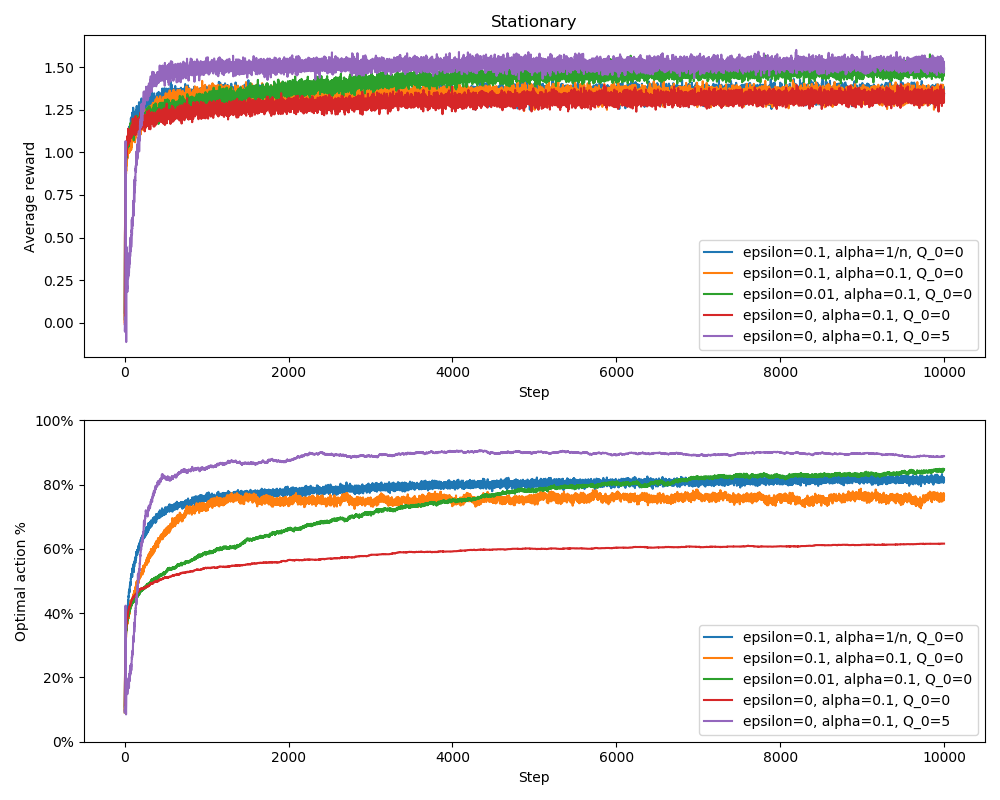
The greedy method with estimates initialized to 0 ($Q_0=0$) performed the worst. It can be hard to see in the reward plot, but it performed slightly worse than the $\epsilon$-greedy methods with $\epsilon=0.1$. Of the $\epsilon$-greedy methods with $\epsilon=0.1$, the one with $\alpha=1/N(a)$ performed slightly better than the one with a constant $\alpha=0.1$. The $\epsilon$-greedy method with $\epsilon=0.01$ takes a long time before it gets good since it explores only 1% of the time. Eventually it learns good enough estimates and overtakes the other $\epsilon$-greedy methods since it selects sub-optimal actions less.

The optimal action percentage plot is easier to read and it clearly shows why the greedy method with $Q_0=0$ performed the worst. It does not explore at all and misses out on selecting the optimal action a lot. However, the greedy method with $Q_0=5$ actually performed the best. The reason is that the high initial estimates forces the agent to try out all actions in the beginning, and thus learns good value estimates. After value estimates are learned, the purely greedy method has the advantage of never selecting actions with lower value estimates. This trick is called optimistic initial values and a similar effect can be achieved by an $\epsilon$-greedy method with large initial $\epsilon$ that reduces to 0 after some time.

Plots for the non-stationary problems:

This time the greedy method with $Q_0=5$ did not perform as good. It starts out by learning good value estimates, but can’t adapt to the changing values. This can be seen by the decreasing optimal action percentage. The $\epsilon$-greedy method with $\alpha=1/N(a)$ performed much worse on the non-stationary version as predicted. Since the updates to the value estimates gets smaller and smaller, it can’t adapt to the changing values.

There are many other action-value methods, such as methods using Upper-Confidence-Bound action selection (UCB). When estimating values there are varying degrees of uncertainty, depending on how often an action has been taken. UCB quantifies this uncertainty as confidence bounds around value estimates and uses these when selecting actions. There are also methods that doesn’t use value estimates, such as gradient bandit algorithms.

Conclusion

This has been a short introduction to multi-armed bandits. The model is simple but can be used for modelling repeated decision problems in the real world. An example of such a problem could be clinical trials where the effect of different drugs on patients with the same illness are compared. For each patient it has to be decided what drug to treat them with. The reward could be 1 if the patient recovers and 0 otherwise. Multi-armed bandits are also useful for introducing important concepts in RL, such as value estimation and the exploration vs exploitation tradeoff.

Thank you for reading and feel free to send me any questions.