import numpy as np
rng = np.random.default_rng(seed=7)
from sklearn.linear_model import LinearRegression
NUM_DATA_POINTS = 100000
Introduction
I just finished studying Brady Neal's Introduction to Causal Inference course. It was a great introduction to the topic for me, and the author was kind enough to release both the lectures and the associated course book for free (at the time of writing this there were a few chapters not yet published). The main goal of this article is to get my hands dirty and solidify some of the things I learned - it would be a nice bonus if it turns out helping someone else as well! You can find the source for this exported notebook in this repository.
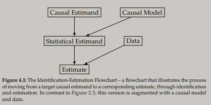
Let's start off with some semantics. Figure 4.1 from the course book illustrates a general procedure of causal inference: the flow from a causal estimand + causal model to a statistical estimand, and from a statistical estimand + data to an estimate. Here are some relevant terms, using the definitions from the Introduction to Causal Inference-book:
- Causal estimand
- The causal expression we are interested in evaluating. Can not be directly estimated from data.
- Contains one or more potential outcomes or $do$-operators, e.g. $\mathbb{E}[Y(t)] = \mathbb{E}[Y|do(T=t)]$.
- Both sides of the equality can be read as "the expected value of the outcome variable $Y$, given that the population of interest receives treatment $T=t$". The left side utilizes potential outcome notation and the right side $do$-operator notation.
- Note that "receives treatment" doesn't have to mean a designed intervention in this context, see Does Obesity Shorten Life? Or is it the Soda? On Non-manipulable Causes (Pearl, 2018) for more information.
- In this article I will primarily consider the specific causal estimand average treatment effect (ATE): $E[Y(1) - Y(0)] = E[Y|do(T=1)] - E[Y|do(T=0)]$. I will focus on the case where the treatment is binary, with $T=1$ denoting treatment and $T=0$ no treatment. However, most of the concepts I will cover easily extend to the continuous treatment case.
- Statistical estimand
- Unlike causal estimands, statistical estimands contain no potential outcomes or $do$-operators and can be estimated from data. Therefore a big part of causal inference is identification - the process of moving from a causal estimand to a statistical estimand. Note that causal estimands are not always identifiable.
- What statistical estimand is a proper identification of the causal estimand of interest (and if it's identifiable at all) depends on the causal model. Causal models are commonly visualized by a directed acyclic graph (DAG) and/or specified by a structural casual model (SCM).
- Estimate (noun)
- An approximation of the estimand we want to estimate (verb) - a concrete value or distribution. The outcome of estimating a statistical estimand using data.
- An estimator is a function that maps from a dataset to an estimate of the (statistical) estimand we are considering.
- There are many ways to do estimation. In this article I will focus on conditional outcome modeling (COM). Other types of methods include, but are not limited to:
- Matching methods
- Inverse probability weighting
- Double machine learning
- Causal trees and forests
Causal model
When working with observational data and attempting to make causal inferences, thinking about the underlying causal model that generated the data is essential (in the experimental setting, when running well designed randomized controlled trials, it's less important due to the random selection into treatment and control groups that makes sure there is no confounding). Association does not imply causation, due to the fact that association doesn't have a direction (e.g. a rooster's crow is associated with the sun rising, but is not the cause of it), and due to the possibility of confounding variables that have an effect on both treatment and outcome variables (e.g. eating ice cream is probably associated with drowning, since going to the beach increases the probability of both ice cream consumption and drowning). One might be tempted (many researchers have been) to simply control for as many covariates as possible in order to reduce the probability of significant confounding. However, the section about colliders will explain why this can be a bad strategy.
Graphical causal model
Graphical models can be utilized to visualize causal relationships between variables. Commonly used are DAGs, where each node represents a variable and each edge a causal relationship. An edge from $A$ to $B$ means that $A$ is a cause of $B$. You can read more about causal graphs in chapters 3 and 4 of the Introduction to Causal Inference-book. The simple DAG below (copied from the book) has a common structure, where treatment $T$ is a cause of outcome $Y$, and confounder $W$ is a common cause of both $T$ and $Y$. We are usually interested in the causal effect of the treatment on the outcome.

Structural causal model
Graphical causal models are very useful, but SCMs can bring additional clarity and allow us to compute counterfactuals. You can read about SCMs in section 4.5 of the Introduction to Causal Inference-book, where they are defined as:
A structural causal model is a tuple of the following sets:
- A set of endogenous variables $V$
- A set of exogenous variables $U$
- A set of functions $f$, one to generate each endogenous variable as a function of other variables
Endogenous variables are variables with at least one parent in the corresponding causal graph, i.e. the variables we are modeling the causes of. Exogenous variables are the variables without parents in the causal graph. An example from the book are the following structural equations

that correspond to the following DAG
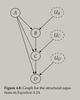
Note that unlike "$=$", "$:=$" is directional - assymetry is needed to describe causal relationships. Here the endogenous variables are $\{B,C,D\}$ and the exogenous variables are $\{A,U_B,U_C,U_D\}$. The set $\{U_B,U_C,U_D\}$ are random noise variables that make the endogenous variables random variables, even if all functions in $f$ are deterministic. The noise variables are usually ommited from DAGs but are shown here to clarify the connection to the SCM.
Below are the structural equations for the DAG presented earlier
Data generating process
We are going to use these structural equations to generate some data, in this case with
$$ \begin{aligned} f_W(U_W) &= \text{Bernoulli}(0.5) \\ f_T(W, U_T) &= H\big(0.8 W + \mathcal{N}(0,1)\big) \\ f_Y(W, T, U_Y) &= 1.5 W - 0.1 T + \mathcal{N}(0,1) \end{aligned} $$where $\mathcal{N}(0,1)$ is the standard normal distribution, and $H(x)$ is the Heaviside step function defined as
$$ H(x) := \begin{cases} 1, & x \geq 0 \\ 0, & x < 0 \end{cases} $$def f_w():
u_w = rng.choice([0, 1])
return u_w
def f_t(w):
u_t = rng.normal()
intermediate = 0.8 * w + u_t
return 1 if intermediate >= 0 else 0
def f_y(w, t):
u_y = rng.normal()
return 1.5 * w - 0.1 * t + u_y
W = np.array([f_w() for _ in range(NUM_DATA_POINTS)])
T = np.array([f_t(w) for w in W])
Y = np.array([f_y(w, t) for w, t in zip(W, T)])
Since we generated the data, we know the true ATE to be $E[Y|do(T=1)] - E[Y|do(T=0)] = -0.1$ (we will of course not know the true ATE in practice). We can estimate the associational difference $E[Y|T=1] - E[Y|T=0]$
np.average(Y[T == 1]) - np.average(Y[T == 0])
0.36637940097327165
We can see that $E[Y|T=1] - E[Y|T=0] \neq E[Y|do(T=1)] - E[Y|do(T=0)]$, due to the confounder $W$. An example showing that association is not causation in general.
Identification
In any DAG, causal association flows through directed paths from $T$ to $Y$. In the case of the specific DAG we have been working with so far, it's particularily simple. The causal association flows directly $T \rightarrow Y$ without any mediators (an example of a mediator is $B$ in the "chain" path $A \rightarrow B \rightarrow C$, since $A$ only affects $C$ through $B$). The non-causal association flows through the backdoor path of $T \leftarrow W \rightarrow Y$. An example of a backdoor path is the ice cream scenario mentioned in the Introduction. You can imagine $T$ as eating ice cream, $Y$ as drowning, and $W$ as being on the beach. Being on the beach increases the probability of both $T$ and $Y$, and thus makes them associated in a non-causal manner.
We are interested in the causal association between $T$ and $Y$, and therefore we have to block the backdoor path. In this case it's simple, since $W$ satisfies what's called the backdoor criterion. A set of variables $W$ satisfies the backdoor criterion relative to $T$ and $Y$ if the following are true:
- $W$ blocks all backdoor paths from $T$ to $Y$.
- $W$ does not contain any descendants of $T$.
The first part of the criterion is quite natural, but the second part is probably less intuitive. We are going to give it more attention in the section about colliders. Assuming that we have modularity and positivity (Assumptions 4.1 and 2.3 in the Introduction to Causal Inference-book), when a set of variables $W$ satisfy the backdoor criterion (relative to $T$ and $Y$), we can utilize the backdoor adjustment to isolate the causal association between $T$ and $Y$:
$$ P(y|do(t)) = \sum_{w} P(y|t,w)P(w) $$Where we are summing over all the possible sets of values for $W$, and $P(w)$ is the probability of observing the set of values $w$ (in the data we have generated, $W$ is a single variable). The backdoor adjustment is more general, but closely related to the adjustment formula for potential outcomes when we have conditional exchangeablity (you can read more about potential outcomes in chapter 2 of the Introduction to Causal Inference-book):
$$ \mathbb{E}[Y(1)-Y(0)] = \mathbb{E}_W\big[\mathbb{E}[Y|T=1,W]-\mathbb{E}[Y|T=0,W]\big] $$We have conditional exchangeability when the units/individuals that we study are comparable within some groups, e.g. grouping by values of $W$. I.e. when there is no confounding within values of $W$, which is the case for the DAG we have been using as an example. Showing the connection between the adjustment formula and the backdoor adjustment just needs a few steps:
$$ \begin{aligned} P(y|do(t)) &= \sum_{w} P(y|t,w)P(w) \\ \sum_y y P(y|do(t)) &= \sum_y y \sum_{w} P(y|t,w)P(w) \\ \mathbb{E}[Y|do(t)] &= \mathbb{E}_W\big[\mathbb{E}[Y|t,W]\big] \\ \mathbb{E}[Y|do(1)] - \mathbb{E}[Y|do(0)] &= \mathbb{E}_W\big[\mathbb{E}[Y|T=1,W] - \mathbb{E}[Y|T=0,W]\big] \\ \mathbb{E}[Y(1) - Y(0)] &= \mathbb{E}_W\big[\mathbb{E}[Y|T=1,W] - \mathbb{E}[Y|T=0,W]\big] \end{aligned} $$As a bonus, in the last two steps we have two different notations for the ATE (the causal estimand we want to estimate) on the left side of the equalities, and an identified statistical estimand on the right side. Therefore, we are now ready for estimation. Note that there are many other concepts when it comes to identifying causal effects, but the backdoor adjustment is one of the most important.
Estimation
We have now identified the ATE:
$$ \begin{aligned} \mathbb{E}[Y|do(1)] - \mathbb{E}[Y|do(0)] &= \mathbb{E}_W\big[\mathbb{E}[Y|T=1,W] - \mathbb{E}[Y|T=0,W]\big] \\ &= \mathbb{E}_W\big[\mathbb{E}[Y|T=1,W]\big] - \mathbb{E}_W\big[\mathbb{E}[Y|T=0,W]\big] \end{aligned} $$We can fit a linear regression model to our generated data, to estimate $\mathbb{E}_W\big[\mathbb{E}[Y|T,W]\big]$. We can then use that model (estimator) to compute an estimate of the ATE. Note that while we know that a linear model is approriate in this case because we have full knowledge about the data generating process, this is not true in general. Assuming linear functions in the SCM is a big, but common assumption that might or might not be appropriate depending on the problem at hand. There are many estimation methods in causal inference, what we are using here is a type of conditional outcome modeling (COM). You can read more about estimation in chapter 7 of the Introduction to Causal Inference-book.
WT = np.array([W, T]).T
WT_1 = np.array([W, np.ones(len(W))]).T
WT_0 = np.array([W, np.zeros(len(W))]).T
model = LinearRegression()
model.fit(WT, Y)
ate_estimate = np.mean(model.predict(WT_1) - model.predict(WT_0))
print("ATE estimate:", ate_estimate)
ATE estimate: -0.10433812966782054
Unlike when using the naive associational difference earlier, we now get an estimate close to the true ATE -0.1 (the difference is due to the randomness in the data generation). Since we are using a linear model, we get an equivalent estimate by simply looking at the slope coefficient.
print("ATE estimate:", model.coef_[1])
ATE estimate: -0.10433812966782059
Colliders
The second part of the backdoor criterion says "$W$ does not contain any descendants of $T$". This is because if we condition on descendants of $T$, we risk condition on a collider. Conditioning on colliders is bad because it opens up new paths for non-causal association to flow between $T$ and $Y$. Consider the following DAG where we have added a new variable $Z$.

Without conditioning on $Z$, association only flows between $T$ and $Y$ through the paths $T \rightarrow Y$ (causal association) and $T \leftarrow W \rightarrow Y$ (non-causal association). When we condition on $Z$, we open up a new non-causal path for association to flow through from $T$ to $Y$. To see why this is the case, it's probably easiest to think of an example. Imagine that we have a simplified model of student success, with $T$ denoting talent for studying, $Y$ propensity to work hard, and $Z$ how hard it is to get in to the student's university. Let's say that there is no causal effect from $T$ to $Y$, but that both variables have a positive causal effect on $Z$. I.e. both more talent and more hard work increase the likelihood of getting admitted to higher ranked universities. A teacher in a low ranked university might conclude that talented students work less hard in general, due to that most students that are both talented and have a high propensity for hard work will be in higher ranked universites. In this scenario the teacher has essentially conditioned on the collider $Z$, opening up a path of non-causal association $T \rightarrow Z \leftarrow Y$.
Let's keep the new SCM the same as the previous one, except for the addition of $Z$ and $f_Z$:
$$ \begin{aligned} W &:= f_W(U_W) = \text{Bernoulli}(0.5) \\ T &:= f_T(W, U_T) = H\big(0.8 W + \mathcal{N}(0,1)\big) \\ Y &:= f_Y(W, T, U_Y) = 1.5 W - 0.1 T + \mathcal{N}(0,1) \\ Z &:= f_Z(T, Y, U_Z) = t - y + \mathcal{N}(0,1) \end{aligned} $$def f_w():
u_w = rng.choice([0, 1])
return u_w
def f_t(w):
u_t = rng.normal()
intermediate = 0.8 * w + u_t
return 1 if intermediate >= 0 else 0
def f_y(w, t):
u_y = rng.normal()
return 1.5 * w - 0.1 * t + u_y
def f_z(t, y):
u_z = rng.normal()
intermediate = t - y + u_z
return 1 if intermediate > 0 else 0
W = np.array([f_w() for _ in range(NUM_DATA_POINTS)])
T = np.array([f_t(w) for w in W])
Y = np.array([f_y(w, t) for w, t in zip(W, T)])
Z = np.array([f_z(t, y) for t, y in zip(T, Y)])
WZT = np.array([W, Z, T]).T
WZT_1 = np.array([W, Z, np.ones(len(W))]).T
WZT_0 = np.array([W, Z, np.zeros(len(W))]).T
model = LinearRegression()
model.fit(WZT, Y)
ate_estimate = np.mean(model.predict(WZT_1) - model.predict(WZT_0))
print("ATE estimate:", ate_estimate)
ATE estimate: 0.2171596888208843
We can see how conditioning on the collider $Z$ makes our estimate move away from the true ATE, which is still -0.1. If we simply omit $Z$ from our conditioning set, we will once again get a good estimate:
WT = np.array([W, T]).T
WT_1 = np.array([W, np.ones(len(W))]).T
WT_0 = np.array([W, np.zeros(len(W))]).T
model = LinearRegression()
model.fit(WT, Y)
ate_estimate = np.mean(model.predict(WT_1) - model.predict(WT_0))
print("ATE estimate:", ate_estimate)
ATE estimate: -0.09518796549143996
Unobserved confounding
So far we have only considered situations where all confounders are observed. We know that this is the case, since we know how the data was generated. In the real world we won't know whether we missed any variables that should be conditioned on - no unobserved confounding is an untestable assumption. To the first DAG we considered, let's add a variable $U$ that like $W$ confounds the casual effect of $T$ on $Y$, but unlike $W$ is not observed.

Here is the new SCM:
$$ \begin{aligned} W &:= f_W(U_W) = \text{Bernoulli}(0.5) \\ U &:= f_U(U_U) = \mathcal{N}(0,1) \\ T &:= f_T(W, U, U_T) = H\big(0.8 W + 1.2 U + \mathcal{N}(0,1)\big) \\ Y &:= f_Y(W, U, T, U_Y) = 1.5 W + 1.1 U - 0.1 T + \mathcal{N}(0,1) \\ \end{aligned} $$def f_w():
u_w = rng.choice([0, 1])
return u_w
def f_u():
u_u = rng.normal()
return u_u
def f_t(w, u):
u_t = rng.normal()
intermediate = 0.8 * w + 1.2 * u + u_t
return 1 if intermediate >= 0 else 0
def f_y(w, u, t):
u_y = rng.normal()
return 1.5 * w + 1.1 * u - 0.1 * t + u_y
W = np.array([f_w() for _ in range(NUM_DATA_POINTS)])
U = np.array([f_u() for _ in range(NUM_DATA_POINTS)])
T = np.array([f_t(w, u) for w, u in zip(W, U)])
Y = np.array([f_y(w, u, t) for w, u, t in zip(W, U, T)])
WT = np.array([W, T]).T
WT_1 = np.array([W, np.ones(len(W))]).T
WT_0 = np.array([W, np.zeros(len(W))]).T
model = LinearRegression()
model.fit(WT, Y)
ate_estimate = np.mean(model.predict(WT_1) - model.predict(WT_0))
print("ATE estimate:", ate_estimate)
ATE estimate: 1.2610170425806635
Our estimate of the ATE is way off the true ATE (still -0.1), showing how unobserved confounding can make causal inferences completely innacurate.
Sensitivity analysis
Since we won't know whether we have unobserved confounding in practice, a common question is how robust our conclusion is to unobserved confounding. E.g. if we estimate that the casual effect of the treatment on the outcome is positive, how much unobserved confounding has to be present for the true effect to be non-positive. While very important, sensitivity analysis is a big and complex topic that I won't go into in this article. You can read a bit about in section 8.2 in the Introduction to Causal Inference-book, but it's a short section that leaves questions unanswered. It does however contain many references to important papers that you can check out if you want to dive deeper.
Conclusion
This has been a brief introduction to some of the basic concepts of causal inference. If you're looking to learn more, I encourage you to check out Introduction to Causal Inference or Which causal inference book you should read (a blog post also written by Brady Neal). I hope you got something out of this article, and feel free to reach out if you have any questions!