Regression Techniques

Introduction

Regression is an important part of Machine Learning, where one tries to find an underlying function that is a good fit to some noisy data. As an example, you might want to predict how much you could sell a house for given data from other house sales. The data would contain input/output pairs of house features (such as size, number of rooms, location, etc.) and corresponding price.

I have implemented two models in TensorFlow, one using simple linear regression and another using a shallow feedforward neural network (FNN). For visualization purposes, I decided to only use one dimensional data, but the code can easily be adapted to data with multiple dimensions.

The source code can be found at https://github.com/CarlFredriksson/regression_techniques.

Implementation

Import Modules

We will need to import the following modules:

import os
import numpy as np
import tensorflow as tf
import matplotlib.pyplot as plt

Generate Data

Since this project is only a proof of concept, I decided to use generated training data instead of looking for some real world data.

def generate_random_data(a=1, b=2, non_linear=False, noise_stdev=1):
    """Generate data with random noise."""
    X = np.expand_dims(np.linspace(-5, 5, num=50), axis=1)
    Y = a * X + b
    if non_linear:
        Y = a * X**2 + b
    noise = np.random.normal(0, noise_stdev, size=X.shape)
    Y += noise
    Y = Y.astype("float32")

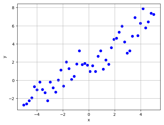
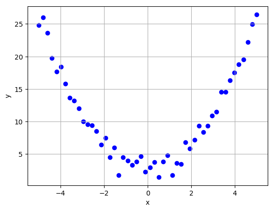
    return X, Y

The function can generate linear data of the form $y=ax+b$ and non-linear data of the form $y=ax^2+b$. I used $a=1$ and $b=2$ for all data sets.

Let us generate some training data that will be used to train the models.

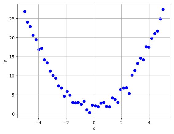
Let us also generate some test data that will be used to evaluate the models.

Linear Regression

The first model I implemented used simple linear regression. This technique assumes that the underlying function is of the form $y=ax+b$, and the objective is to find the values for $a$ and $b$ that best fit the data. We need to define a cost function that makes us achieve this objective, and a very common one is squared error cost. Let us define $m$ as the number of training examples, $X_{train}$ as the input features, and $Y_{train}$ as the correct outputs for those features. Both $X_{train}$ and $Y_{train}$ have the dimensions $(m,1)$. Let us also define $Y_{estimate}$ as the values we get using our estimated $a$ and $b$ values ($a_{estimate}$ and $b_{estimate}$). The cost is defined as:

$$ J(X_{train}, Y_{train}, Y_{estimate}) = \frac{1}{m} \sum_{x \in X_{train}} (Y_{train}(x) - Y_{estimate}(x))^2 $$

or in other words:

$$ J(X_{train}, a, b, a_{estimate}, b_{estimate}) = \frac{1}{m} \sum_{x \in X_{train}} ((ax+b) - (a_{estimate}x+b_{estimate}))^2 $$

def linear_regression_1D(X_train, Y_train, X_test, Y_test, learning_rate, num_iterations):
    y_est = []

    # Create parameters
    a_estimate = tf.Variable(0, dtype=tf.float32)
    b_estimate = tf.Variable(0, dtype=tf.float32)

    # Compute cost
    X_placeholder = tf.placeholder(dtype=tf.float32, shape=(None, 1), name="X_placeholder")
    Y_placeholder = tf.placeholder(dtype=tf.float32, shape=(None, 1), name="Y_placeholder")
    Y_estimate = a_estimate * X_placeholder + b_estimate
    J = tf.reduce_mean((Y_placeholder - Y_estimate)**2)

    # Create train op
    optimizer = tf.train.GradientDescentOptimizer(learning_rate)
    train_op = optimizer.minimize(J)

    # Start session
    with tf.Session() as sess:
        # Initialize variables
        sess.run(tf.global_variables_initializer())

        # Training loop
        for i in range(num_iterations):
            sess.run(train_op, feed_dict={X_placeholder: X_train, Y_placeholder: Y_train})

        # Create estimated Y values
        y_est, J_train = sess.run([Y_estimate, J], feed_dict={X_placeholder: X_train, Y_placeholder: Y_train})
        J_test = sess.run(J, feed_dict={X_placeholder: X_test, Y_placeholder: Y_test})

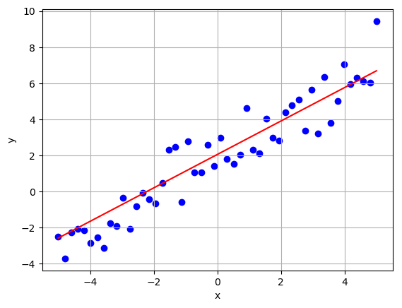
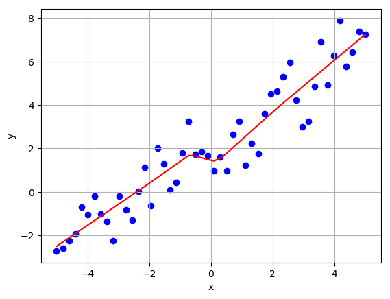
    return y_est, J_train, J_test

As one might expect, this simple model yielded a good result when applied to our generated linear data. It fit the training set pretty well with a final cost of 0.9422.

More importantly, it also had good results on the test set with a final cost of 1.0851.

However, when the model is used on a non-linear data set, it obviously fails miserably. On the training set the final cost was 53.182.

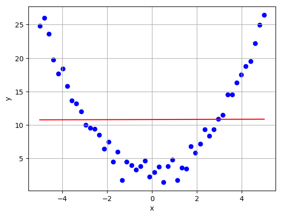
On the test set the final cost was 62.886.

Neural Network Regression

The second model I implemented uses a small FNN. The network has two hidden layers with ten neurons each. ReLU is used as an activation function for all layers except the output layer, which has a single linear neuron. Note that if the hidden layers are removed, we are left with simple linear regression. I used the same cost function as in the first model.

def nn_regression_1D(X_train, Y_train, X_test, Y_test, learning_rate, num_iterations):
    tf.reset_default_graph()
    y_est = []
    
    # Create parameters
    W_1 = tf.get_variable("W_1", shape=(1, 10), initializer=tf.contrib.layers.xavier_initializer())
    b_1 = tf.get_variable("b_1", shape=(1, 10), initializer=tf.zeros_initializer())

    W_2 = tf.get_variable("W_2", shape=(10, 10), initializer=tf.contrib.layers.xavier_initializer())
    b_2 = tf.get_variable("b_2", shape=(1, 10), initializer=tf.zeros_initializer())

    W_3 = tf.get_variable("W_3", shape=(10, 1), initializer=tf.contrib.layers.xavier_initializer())
    b_3 = tf.get_variable("b_3", shape=(1, 1), initializer=tf.zeros_initializer())

    # Forward propagation
    X_placeholder = tf.placeholder(dtype=tf.float32, shape=(None, 1), name="X_placeholder")
    Y_placeholder = tf.placeholder(dtype=tf.float32, shape=(None, 1), name="Y_placeholder")

    X = tf.matmul(X_placeholder, W_1) + b_1
    X = tf.nn.relu(X)
    X = tf.matmul(X, W_2) + b_2
    X = tf.nn.relu(X)
    Y_estimate = tf.matmul(X, W_3) + b_3

    # Compute cost
    J = tf.reduce_mean((Y_placeholder - Y_estimate)**2)

    # Create training operation
    optimizer = tf.train.GradientDescentOptimizer(learning_rate)
    train_op = optimizer.minimize(J)

    # Start session
    with tf.Session() as sess:
        # Initialize variables
        sess.run(tf.global_variables_initializer())

        # Training loop
        for i in range(num_iterations):
            sess.run(train_op, feed_dict={X_placeholder: X_train, Y_placeholder: Y_train})

        # Create estimated Y values
        y_est, J_train = sess.run([Y_estimate, J], feed_dict={X_placeholder: X_train, Y_placeholder: Y_train})
        J_test = sess.run(J, feed_dict={X_placeholder: X_test, Y_placeholder: Y_test})
    
    return y_est, J_train, J_test

The FNN model also yielded a good result when applied to our generated linear data. It fit the training set even better than the first model with a final cost of 0.7937.

However, it had worse performance on the test set with a final cost of 1.1286, which is slightly higher than for the first model. This significant difference between performance on the training and test sets are due to overfitting. Overfitting can be combatted by introducing regularization/dropout, getting more data, and/or reducing the size of the network.

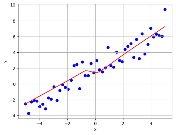
The second model shows its strength when used on the non-linear data set. Since it does not assume the form of the underlying function, it can fit to non-linear data as well. The final cost on the training set was 1.0929.

It once again did some overfitting, and the final cost on the test set was 1.6068.

Conclusion

A simple linear regression model can be a good choice when you are absolutely sure that the underlying function is linear. Otherwise I would use a neural network or a similarly flexible model. You might have to put in more work to find a good network architecture and to avoid overfitting, but you do not have to worry about the possible non-linearity of your data set.

The source code can be found at https://github.com/CarlFredriksson/regression_techniques.

Thank you for reading, and feel free to send me any questions.