Regression using Keras

Introduction

I have started experimenting with Keras, which is a high-level neural networks API. It provides an interface on top of TensorFlow, CNTK, or Theano. So far have been using Keras with TensorFlow as a backend. Keras makes prototyping and experimentation faster and easier, while removing some of the flexibility that TensorFlow has. If you use the TensorFlow backend you can combine the two when the need arises for functionality that Keras does not provide on its own.

In this blog post I am going to show you how to implement simple regression in Keras. We are implementing linear regression as a baseline model, and a small feedforward neural network as a more complex model. For more information about regression, and how to implement it in TensorFlow, check out my previous post Regression Techniques.

The source code can be found at https://github.com/CarlFredriksson/regression_using_keras.

Implementation

Import Modules

We will need to import the following modules:

import numpy as np
import matplotlib.pyplot as plt
from keras.models import Sequential
from keras.layers import Dense
from keras.optimizers import SGD

Generate Data

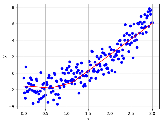
Since this project is only a proof of concept, I decided to use randomly generated datasets. The generated data is of the form $y=x^2-2$ for $0 \leq x \leq 3$ with some normally distributed random noise added to simulate real world data.

def generate_random_data():
    X = np.expand_dims(np.linspace(0, 3, num=200), axis=1)
    Y = X**2 - 2
    noise = np.random.normal(0, 1, size=X.shape)
    Y = Y + noise
    Y = Y.astype("float32")
    return X, Y

Let us generate datasets for training and validation.

X_train, Y_train = generate_random_data()
X_val, Y_val = generate_random_data()

To visualize the datasets we can plot them using Matplotlib.

def plot_data(X, Y, plot_name):
    plt.scatter(X, Y, color="blue")
    plt.grid()
    plt.xlabel("x")
    plt.ylabel("y")
    plt.savefig("output/" + plot_name, bbox_inches="tight")
    plt.clf()

plot_data(X_train, Y_train, "data_train.png")
plot_data(X_val, Y_val, "data_val.png")

Create Baseline Model

To implement simple linear regression we can use a neural network without hidden layers. In Keras we use a single dense layer for this. A dense layer is a normal fully connected layer. Note that the first (and only layer in this case) of a sequential Keras model needs to specify the input shape. To finish creating a model we need to compile it, while specifying what optimizer we want and what loss function to use.

def create_baseline_model():
    model = Sequential()
    model.add(Dense(1, input_shape=(1,)))
    model.compile(optimizer=SGD(lr=0.001), loss="mean_squared_error")
    return model

Create More Complex Model

The more complex model will contain three hidden layers of ten neurons each. Do not forget to add an activation function to the hidden layers.

def create_nn_model():
    model = Sequential()
    model.add(Dense(10, input_shape=(1,), activation="relu"))
    model.add(Dense(10, activation="relu"))
    model.add(Dense(10, activation="relu"))
    model.add(Dense(1))
    model.compile(optimizer=SGD(lr=0.001), loss="mean_squared_error")
    return model

Train Models

Training a model in Keras is very simple with the model.fit function. It is one of the nice high level functions that allows us to get up and runnning very quickly. Since the training set I generated is very small, I decided to use the whole set each batch.

history = model.fit(X_train, Y_train, batch_size=X_train.shape[0], epochs=10000, validation_data=(X_val, Y_val))

The model.fit function returns a history of the training and validation losses. To evaluate a model it is often a good idea to plot the history.

def plot_history(history, plot_name):
    plt.plot(history.epoch, np.array(history.history["loss"]), label="Train loss")
    plt.plot(history.epoch, np.array(history.history["val_loss"]), label="Val loss")
    plt.xlabel("Epoch")
    plt.ylabel("Loss (Mean squared error)")
    plt.legend()
    plt.savefig("output/" + plot_name, bbox_inches="tight")
    plt.clf()

For the baseline model:

plot_history(history, "history_baseline.png")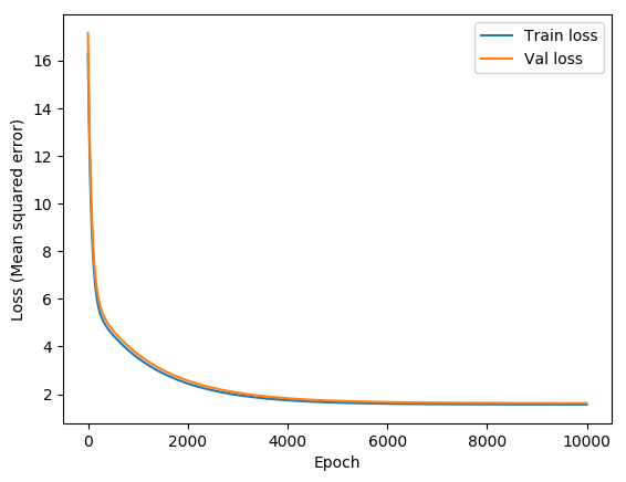

For the more complex model:

plot_history(history, "history_nn.png")

We can also evaluate models using the model.evaluate function. This returns the final loss for the specified dataset.

final_train_loss = model.evaluate(X_train, Y_train, verbose=0)
final_val_loss = model.evaluate(X_val, Y_val, verbose=0)

For the run that resulted in the plots above, the final training and validation losses were 1.566 and 1.621 for the baseline model, 1.080 and 1.184 for the more complex model.

Using the Trained Models

In order to output predictions for a given dataset we can use the model.predict function.

Y_predict = model.predict(X_val)

The predictions can be plotted on top of the data using the following function:

def plot_results(X, Y, Y_predict, plot_name):
    plt.scatter(X, Y, color="blue")
    plt.plot(X, Y_predict, color="red")
    plt.grid()
    plt.xlabel("x")
    plt.ylabel("y")
    plt.savefig("output/" + plot_name, bbox_inches="tight")
    plt.clf()

For the baseline model:

plot_results(X_val, Y_val, Y_predict, "results_baseline.png")

For the more complex model:

plot_results(X_val, Y_val, Y_predict, "results_nn.png")

Conclusion

Keras is a powerful library that lets developers iterate quickly. For this simple project there was no need for deep networks, but Keras was developed with deep learning in mind, and is well suited for creating deeper and more complex models.