Temporal Difference Learning

Introduction

“If one had to identify one idea as central and novel to reinforcement learning, it would undoubtedly be temporal-difference (TD) learning” (Reinforcement Learning: An Introduction, Sutton, Barto, 2018).

TD learning combines ideas from Monte Carlo Methods (MC methods) and Dynamic Programming (DP). Like DP and MC methods, TD methods are a form of generalized policy iteration (GPI), which means that they alternate policy evaluation (estimation of value functions) and policy improvement (using value estimates to improve a policy). Like MC methods, TD methods don’t need to know the underlying dynamics of the model and instead learn from experience. Unlike MC methods but like DP, TD methods use bootstrapping, which means that value estimates are updated using other value estimates.

Unlike MC methods, which update value estimates and the target policy after each episode, TD methods update estimates and the target policy after each time step. This makes TD methods work on continuous tasks as well as episodic tasks. On episodic tasks, where MC methods can work as well, TD methods usually converge faster.

The aim of this article is to be a short introduction to TD learning. To read more about this subject, I recommend (Sutton, Barto, 2018). Later in the article there is going to be an implemented example of a couple of TD methods that solves a gridworld problem. The source code can be found at https://github.com/CarlFredriksson/temporal_difference_learning.

Sarsa

Sarsa is an on-policy TD method that uses action-value estimates $Q_\pi(s,a)$ to improve the target policy $\pi$. To assure that the agent explores sufficiently, the policy $\pi$ has to be soft, which means that all actions in every state has a probability greater than zero of being selected. A commonly used type of soft policies are $\epsilon$-greedy policies that select the action that maximizes $Q_\pi(s,a)$ with probability $1-\epsilon$ and a random action with probability $\epsilon$.

In Sarsa, the action-value estimates are improved using the update rule

The name Sarsa comes from the fact that $S_t,A_t,R_{t+1},S_{t+1},A_{t+1}$ are used in the update rule, which spells out SARSA if the subscripts are dropped.

Pseudocode for Sarsa with the target policy being any soft policy derived from $Q$ (e.g. $\epsilon$-greedy) is given below.

Q-learning

Q-learning is an off-policy TD method. Thus, it uses two different policies, the the target policy $\pi$ and the behavior policy $b$. The target policy is used for value estimation and is the target for improvement, while the behavior policy is used for action selection. The behavior policy has to be soft in order to maintain sufficient exploration. The target policy can be completely greedy.

In Q-learning, the action-value estimates are improved using the update rule

The name Q-learning simply comes from the use of action value estimates $Q$.

Pseudocode for Q-learning with the target policy being the greedy policy derived from $Q$ and the behavior policy being any soft policy derived from $Q$ (e.g. $\epsilon$-greedy) is given below.

Windy Gridworld Example

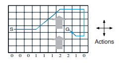
We are going to use Example 6.5: Windy Gridworld (Sutton, Barto, 2018) as a problem for showcasing Python implementations of Sarsa and Q-learning. It is a standard gridworld problem with the addition of wind that moves the agent upward a different number of cells depending on which column the agent is on after taking an action. The state is the cell position of the agent and the available actions are UP, DOWN, LEFT, RIGHT in every state. The actions deterministically move the agent in their respective directions before wind is applied. If the agent would move outside of the gridworld (by an action or by the wind), it stays in same cell as before moving. The task is episodic and undiscounted with a reward of -1 given after every action, except when the goal state G is reached. The gridworld is visualized in the following image, with the blue line representing the optimal trajectory when starting from state S.

Note that MC methods cannot easily be used for this problem since not all policies are guaranteed to end up in a terminal state (the goal state). This can lead to infinite episodes if the number of steps isn’t limited. TD methods don’t have the same problem since they learn during episodes and will eventually end up in the goal state. Below is an implementation of the gridworld environment agents can interact with by calling the take_action function.

class Action(Enum):
    UP = 0
    DOWN = 1
    LEFT = 2
    RIGHT = 3

class Environment:
    def __init__(self, starting_state):
        self.wind = [0, 0, 0, 1, 1, 1, 2, 2, 1, 0]
        self.goal = (7, 3)
        self.state = starting_state

    def adjust_position(self):
        # X position
        if self.state[0] < 0:
            self.state = (0, self.state[1])
        elif self.state[0] > 9:
            self.state = (9, self.state[1])

        # Y Position
        if self.state[1] < 0:
            self.state = (self.state[0], 0)
        elif self.state[1] > 6:
            self.state = (self.state[0], 6)

    def take_action(self, action):
        # Move agent from action
        if action == Action.UP:
            self.state = (self.state[0], self.state[1] + 1)
        elif action == Action.DOWN:
            self.state = (self.state[0], self.state[1] - 1)
        elif action == Action.LEFT:
            self.state = (self.state[0] - 1, self.state[1])
        elif action == Action.RIGHT:
            self.state = (self.state[0] + 1, self.state[1])
        else:
            print("ERROR: INVALID ACTION SELECTED!")
        self.adjust_position()

        # Move agent from wind
        if self.state != self.goal:
            self.state = (self.state[0], self.state[1] + self.wind[self.state[0]])
            self.adjust_position()

        if self.state == self.goal:
            return 0
        return -1

Implementations of a Sarsa agent and a Q-learning agent:

class SarsaAgent:
    def __init__(self, alpha, epsilon):
        self.alpha = alpha
        self.epsilon = epsilon
        self.Q = np.zeros((10, 7, 4))
        self.a = 0

    def step(self, environment):
        # Take action
        s = environment.state
        r = environment.take_action(Action(self.a))
        s_prime = environment.state

        # Select next action and update Q
        a_prime = epsilon_greedy(self.epsilon, self.Q, s_prime)
        self.Q[s[0], s[1], self.a] += self.alpha * (r + self.Q[s_prime[0], s_prime[1], a_prime] - self.Q[s[0], s[1], self.a])
        self.a = a_prime

        # Check if goal has been reached
        if r == 0:
            return True
        return False

class QLearningAgent:
    def __init__(self, alpha, epsilon):
        self.alpha = alpha
        self.epsilon = epsilon
        self.Q = np.zeros((10, 7, 4))

    def step(self, environment):
        # Select action
        s = environment.state
        a = epsilon_greedy(self.epsilon, self.Q, s)

        # Take action
        r = environment.take_action(Action(a))
        s_prime = environment.state

        # Update Q
        self.Q[s[0], s[1], a] += self.alpha * (r + np.max(self.Q[s_prime[0], s_prime[1], :]) - self.Q[s[0], s[1], a])

        # Check if goal has been reached
        if r == 0:
            return True
        return False

def epsilon_greedy(epsilon, Q, s):
    a = np.argmax(Q[s[0], s[1], :])
    if np.random.rand() < epsilon:
        a = np.random.randint(0, 4)
    return a

Some code for running the agents and plotting the results:

if __name__ == "__main__":
    NUM_EPISODES = 200
    MAX_NUM_STEPS = 1000
    ALPHA = 0.5
    EPSILON = 0.1
    STARTING_STATE = (0, 3)

    agents = [
        SarsaAgent(ALPHA, EPSILON),
        QLearningAgent(ALPHA, EPSILON)
    ]
    num_steps = np.zeros((len(agents), NUM_EPISODES))

    # Agents learning
    for agent_index, agent in enumerate(agents):
        for episode in range(NUM_EPISODES):
            environment = Environment(STARTING_STATE)
            for num_steps[agent_index, episode] in range(MAX_NUM_STEPS):
                at_goal = agent.step(environment)
                if at_goal:
                    break

    # Plot results
    plt.plot(range(NUM_EPISODES), num_steps[0, :], label="Sarsa")
    plt.plot(range(NUM_EPISODES), num_steps[1, :], label="Q-learning")
    plt.legend()
    plt.xlabel("Episode")
    plt.ylabel("Number of steps to reach goal")
    plt.show()

Conclusion

We have described two of the most popular TD methods (and reinforcement learning methods in general), the on-policy method Sarsa and the off-policy method Q-learning. They both are one-step, model-free, and tabular TD methods. TD methods can be extended to n-step forms, which link them to MC methods, and to forms that include a model of the environment, which link them to DP. TD methods can also be extended to be non-tabular and instead use various forms of function approximation, for example by using artificial neural networks.

Thank you for reading and feel free to send me any questions.